Texture Classification Using Multi-Block Local Binary Pattern

Quiz

Multi-Block Local Binary Pattern (MB-LBP) is an extension of the Local Binary Pattern (LBP) technique that allows computation on multiple scales efficiently using the integral image. In MB-LBP, an image is divided into nine equally sized rectangles, and a feature is computed for each of these rectangles. This feature is determined by comparing the sum of pixel intensities within each rectangle to that of the central rectangle, similar to how LBP operates.

The calculation of MB-LBP features follows a similar concept to local binary patterns (LBPs), with the key difference being that summed blocks are used instead of individual pixel values.

The scikit image library offers the multiblock_lbp() function within its feature module to compute multi-block local binary patterns.

Using the skimage.feature.multiblock_lbp() function

The skimage.feature.multiblock_lbp() function is used to compute the Multi-Block Local Binary Pattern (MB-LBP) feature descriptor.

Syntax

The syntax of the function is as follows −

skimage.feature.multiblock_lbp(int_image, r, c, width, height)

Parameters

Here are the parameters of this function −

int_image (N, M) array: This parameter represents the input integral image.
r (int): The row-coordinate of the top-left corner of a rectangle containing the feature.
c (int): The column-coordinate of the top-left corner of a rectangle containing the feature.
width (int): The width of one of the nine equal rectangles that will be used to compute a feature.
height (int): The height of one of the nine equal rectangles that will be used to compute a feature.

The function returns an 8-bit MB-LBP feature descriptor as an integer.

Example

First, let's generate an image to demonstrate how MB-LBP works. We'll consider a (9, 9) rectangle divided into (3, 3) blocks, and then apply MB-LBP to it using the multiblock_lbp() function.

from skimage.feature import multiblock_lbp
import numpy as np
from numpy.testing import assert_equal
from skimage.transform import integral_image

# Create a test matrix where the first and fifth rectangles starting
# from the top-left corner clockwise have greater values than the central one.
test_img = np.zeros((9, 9), dtype='uint8')
test_img[3:6, 3:6] = 1
test_img[:3, :3] = 50
test_img[6:, 6:] = 50

# The first and fifth bits should be filled. This correct value will
# be compared to the computed one.
correct_answer = 0b10001000
int_img = integral_image(test_img)

# Compute the MB-LBP code for the specified rectangle
lbp_code = multiblock_lbp(int_img, 0, 0, 3, 3)

print("Computed MB-LBP Code:", bin(lbp_code))
print("Correct MB-LBP Code:", bin(correct_answer))

# Compare the computed value to the correct one using assert_equal
try:
   assert_equal(correct_answer, lbp_code)
   # If the assertion doesn't raise an exception, the values match
   print('Computed value and the correct one are the same.')
except AssertionError:
   # If the assertion raises an exception, the values don't match
   print("Computed value and the correct one are not the same.")

Output

Computed MB-LBP Code: 0b10001000
Correct MB-LBP Code: 0b10001000
Computed value and the correct one are the same.

Example

Now, let's apply the operator to a real image and visualize the results.

from skimage import io, data 
from matplotlib import pyplot as plt
from skimage.feature import multiblock_lbp
from skimage.feature import draw_multiblock_lbp
from skimage.transform import integral_image

# Load a input image
test_img = io.imread('Images/black-doted-butterflies.jpg', as_gray=True)

# Calculate the integral image for efficient computation
int_img = integral_image(test_img)

# Compute the MB-LBP code for a specified rectangle
lbp_code = multiblock_lbp(int_img, 0, 0, 90, 90)

# Draw the MB-LBP visualization on the image
img = draw_multiblock_lbp(test_img, 0, 0, 90, 90, lbp_code=lbp_code, alpha=0.5)# Display the resulting image with MB-LBP visualization
plt.imshow(img)
plt.show()

Output

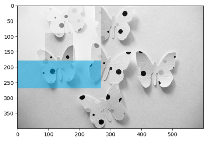
In the plot above, we observe the outcome of computing an MB-LBP feature and visualizing the computed results. The rectangles with a lower sum of intensity values than the central rectangle are highlighted in cyan, while those with higher intensity values are shown in white. The central rectangle remains untouched.

Print Page