Scikit Image - Registration Using Optical Flow

Image registration using optical flow is a computer vision and image processing technique that aims to determine the displacement of pixels between two consecutive image frames in a sequence.

Optical flow is defined as a vector field (u, v) that verifying image1(x+u, y+v) = image0(x, y), where (image0, image1) represents two consecutive 2D frames in a sequence. This vector field is used for image registration through image warping.

This tutorial demonstration the image registration using optical flow.

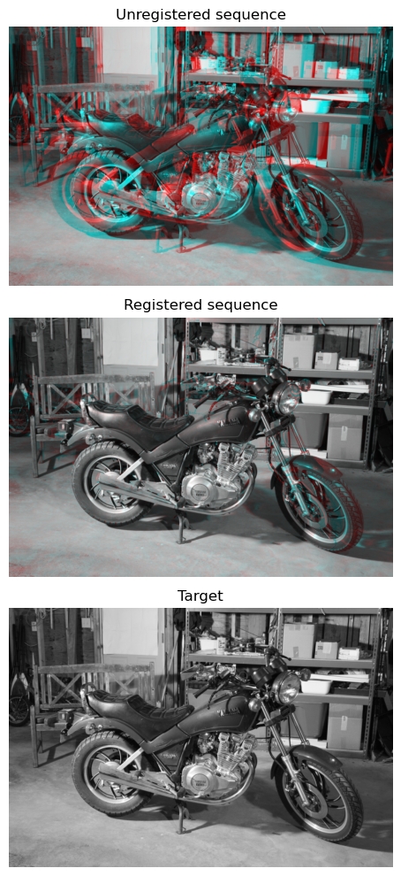
To display registration results, an RGB image is created. The result of the registration is assigned to the red channel, while the target image is assigned to the green and blue channels. A perfect registration results in a gray level image, while misregistered pixels are represented by colors in the constructed RGB image.

Example

The following example demonstrates the process of image registration using optical flow. The function optical_flow_tvl1() is used to estimate the optical flow between the two frames.

import numpy as np
from matplotlib import pyplot as plt
from skimage.color import rgb2gray
from skimage.data import stereo_motorcycle, vortex
from skimage.transform import warp
from skimage.registration import optical_flow_tvl1, optical_flow_ilk

# Load the sequence
first_frame, second_frame, disparity_map = stereo_motorcycle()

# Convert the images to grayscale, as color is not supported
first_frame = rgb2gray(first_frame)
second_frame = rgb2gray(second_frame)

# Compute the optical flow
v, u = optical_flow_tvl1(first_frame, second_frame)

# Define the image grid coordinates
nr, nc = first_frame.shape
row_coords, col_coords = np.meshgrid(np.arange(nr), np.arange(nc), indexing='ij')

# Use the estimated optical flow for registration
second_frame_warp = warp(second_frame, np.array([row_coords + v, col_coords + u]), mode='edge')

# Build an RGB image with the unregistered sequence
unregistered_seq_im = np.zeros((nr, nc, 3))
unregistered_seq_im[..., 0] = second_frame
unregistered_seq_im[..., 1] = first_frame
unregistered_seq_im[..., 2] = first_frame

# Build an RGB image with the registered sequence
registered_seq_im = np.zeros((nr, nc, 3))
registered_seq_im[..., 0] = second_frame_warp
registered_seq_im[..., 1] = first_frame
registered_seq_im[..., 2] = first_frame

# Build an RGB image with the target sequence
target_im = np.zeros((nr, nc, 3))
target_im[..., 0] = first_frame
target_im[..., 1] = first_frame
target_im[..., 2] = first_frame

# Display the results
fig, (ax0, ax1, ax2) = plt.subplots(3, 1, figsize=(5, 10))

ax0.imshow(unregistered_seq_im)
ax0.set_title("Unregistered sequence")
ax0.set_axis_off()

ax1.imshow(registered_seq_im)
ax1.set_title("Registered sequence")
ax1.set_axis_off()

ax2.imshow(target_im)
ax2.set_title("Target")
ax2.set_axis_off()

fig.tight_layout()
plt.show()

Output

Example

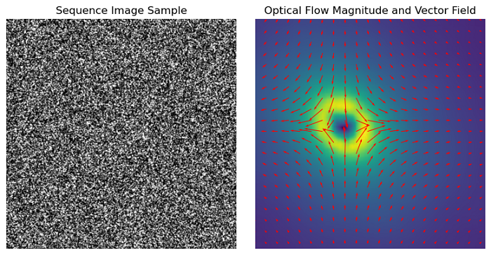
In this example, the "Iterative Lukas-Kanade algorithm (iLK)" is applied to a pair of images, likely capturing the motion of particles or features. It aims to demonstrate how the iLK algorithm can be used to estimate optical flow and visualize motion within an image sequence.

import numpy as np
from matplotlib import pyplot as plt
from skimage.color import rgb2gray
from skimage.data import vortex
from skimage.transform import warp
from skimage.registration import optical_flow_ilk

# Load two images from the 'vortex' dataset
image0, image1 = vortex()

# Compute optical flow using the Iterative Lukas-Kanade algorithm
optical_flow_u, optical_flow_v = optical_flow_ilk(image0, image1, radius=15)

# Compute the magnitude of the optical flow vectors
flow_magnitude = np.sqrt(optical_flow_u ** 2 + optical_flow_v ** 2)

# Create a visualization of the optical flow results
import matplotlib.pyplot as plt

# Set up the subplots
fig, (ax0, ax1) = plt.subplots(1, 2, figsize=(8, 4))

# Display the first image from the sequence
ax0.imshow(image0, cmap='gray')
ax0.set_title("Sequence Image Sample")
ax0.set_axis_off()

# Define parameters for quiver plot
num_vectors = 20  # Number of vectors to be displayed along each dimension
rows, cols = image0.shape
step = max(rows // num_vectors, cols // num_vectors)

# Create coordinates for quiver plot
y, x = np.mgrid[:rows:step, :cols:step]
u_ = optical_flow_u[::step, ::step]
v_ = optical_flow_v[::step, ::step]

# Display optical flow magnitude and vector field using quiver plot
ax1.imshow(flow_magnitude)
ax1.quiver(x, y, u_, v_, color='r', units='dots', angles='xy', scale_units='xy', lw=3)
ax1.set_title("Optical Flow Magnitude and Vector Field")
ax1.set_axis_off()

# Ensure proper layout and display the plot
fig.tight_layout()
plt.show()

Output