Scikit Image - Histogram of Oriented Gradients

Quiz

Histogram of Oriented Gradients, commonly known as HOG, is a widely used image feature descriptor in the field of image processing and computer vision tasks, particularly in the context of object detection. It involves counting occurrences of gradient orientation within localized segments of an image.

The process of computing a Histogram of Oriented Gradients (HOG) descriptors involves several stages −

Global Image Normalization (Optional): As an initial step, there's an optional global image normalization process aimed at reducing the influence of illumination effects. This often involves gamma (power law) compression, such as computing the square root or logarithm of each color channel. This step helps reduce the influence of local shadowing and illumination variations.
Computing the gradient image in x and y: The second stage involves computing first-order image gradients. These gradients capture information related to contours, silhouettes, and some texture details, while also enhancing resistance to variations in illumination.
Computing gradient histograms: The third stage aims to create an encoding sensitive to local image content while remaining robust to minor changes in pose or appearance. This is achieved by pooling gradient orientation information locally in the same way as the SIFT feature. The image is divided into smaller spatial regions known as "cells." For each cell, a local 1-D histogram of gradient or edge orientations is computed using all the pixels within the cell. These individual cell-level histograms collectively form the fundamental "orientation histogram" representation. Each orientation histogram divides the range of gradient angles into a fixed number of predefined bins. The gradient magnitudes of pixels within the cell are used to contribute to the orientation histogram.
Normalising across blocks: In the fourth stage, normalization is applied to enhance invariance to illumination, shadowing, and edge contrast. It's performed by measuring local histogram "energy" over groups of cells known as "blocks" and then normalizing each cell within the block. Each individual cell might be shared across multiple blocks, but its normalizations vary from block to block. As a result, the same cell appears multiple times in the final output vector with different normalizations. This may seem redundant but it improves the performance, and these normalized block descriptors are referred to as Histogram of Oriented Gradient (HOG) descriptors.
Flattening into a feature vector: Finally, HOG descriptors from all blocks in a dense, overlapping grid covering the detection window are combined into a feature vector, which is then used in window classification.

Using the skimage.feature.hog() function

The Scikit-Image provides a flexible implementation of the Histogram of Oriented Gradient (HOG) algorithm with the skimage.feature.hog() function, allowing users to compute HOG features for images with customization options.

Syntax

skimage.feature.hog(image, orientations=9, pixels_per_cell=(8, 8), cells_per_block=(3, 3), block_norm='L2-Hys', visualize=False, transform_sqrt=False, feature_vector=True, *, channel_axis=None)

Parameters

image ((M, N[, C]) ndarray): Input image for which HOG features are computed.
orientations (int, optional): The number of orientation bins.
pixels_per_cell (2-tuple (int, int), optional): The size of a cell in pixels.
cells_per_block (2-tuple (int, int), optional): The number of cells in each block.
block_norm (str {'L1', 'L1-sqrt', 'L2', 'L2-Hys'}, optional): Specifies the block normalization method. Options include −
- 'L1': Normalization using L1-norm.
- 'L1-sqrt': Normalization using L1-norm, followed by square root.
- 'L2': Normalization using L2-norm.
- 'L2-Hys' (default): Normalization using L2-norm, followed by limiting the maximum values to 0.2 (Hys stands for hysteresis) and renormalization using L2-norm.
visualize (bool, optional): If set to True, it returns an image of the HOG features. This image shows line segments for each cell and orientation bin, with intensities proportional to the corresponding histogram values.
transform_sqrt (bool, optional): If set to True, it applies power-law compression to normalize the image before processing. If the image contains negative values then it is recommended to DO NOT use this parameter.
feature_vector (optional): If set to True, it returns the data as a feature vector by calling .ravel() on the result just before returning.
channel_axis (optional): Indicates which axis of the array corresponds to channels in the case of multi-channel images. If None, the image is assumed to be a grayscale (single channel) image.

The function returns two outputs −

Out (n_blocks_row, n_blocks_col, n_cells_row, n_cells_col, n_orient) ndarray: An ndarray representing the HOG descriptor for the image. The shape depends on the parameters and can be multi-dimensional if not flattened. If feature_vector is set to True, a 1D (flattened) array is returned.
hog_image ((M, N) ndarray, optional): An ndarray representing a visualization of the HOG image. This is provided only if visualize is set to True.

Example

Here's an example of how to use the skimage.feature.hog function to compute the Histogram of Oriented Gradients (HOG) features for a color image.

import numpy as np
from skimage import io, feature
import matplotlib.pyplot as plt

# Load the input image
image = io.imread('Images/hand writting.jpg')

# Compute HOG features
hog_features, hog_image = feature.hog(image, orientations=9,
   pixels_per_cell=(8, 8),
   cells_per_block=(3, 3),
   visualize=True, 
   channel_axis=-1)

# Display the original and resultant images
fig, axes = plt.subplots(1, 2, figsize=(10, 8))
ax = axes.ravel()

ax[0].imshow(image, cmap=plt.cm.gray)
ax[0].set_title('Original Image')
ax[0].axis('off')

# Display the HOG visualization
ax[1].imshow(hog_image, cmap=plt.cm.gray)
ax[1].set_title('HOG Visualization')
ax[1].axis('off')
plt.show()

# display the shaope of computed HOG features
print("Shape of HOG features:", hog_features.shape)

Output

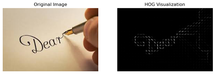
Example

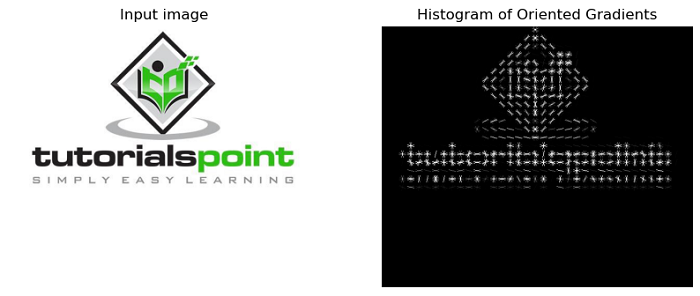
Let's take a different input image and use the feature.hog() function to calculate the Histogram of Oriented Gradients (HOG) features.

import matplotlib.pyplot as plt
from skimage.feature import hog
from skimage import io, exposure

# Load an input image
image = io.imread('Images/logo.jpg')

# Compute HOG features with specified parameters
fd, hog_image = hog(image, orientations=8, pixels_per_cell=(16, 16),
   cells_per_block=(1, 1), visualize=True, channel_axis=-1)

# Create a figure with two subplots
fig, (ax1, ax2) = plt.subplots(1, 2, figsize=(10, 8), sharex=True, sharey=True)

# Display the input image
ax1.axis('off')
ax1.imshow(image, cmap=plt.cm.gray)
ax1.set_title('Input image')

# Rescale histogram for better display
hog_image_rescaled = exposure.rescale_intensity(hog_image, in_range=(0, 10))

# Display the HOG image
ax2.axis('off')
ax2.imshow(hog_image_rescaled, cmap=plt.cm.gray)
ax2.set_title('Histogram of Oriented Gradients')

plt.show()

Output

Print Page