SciPy - signal.lfilter() Function

---

---

scipy.signal.lfilter() is a function in SciPy's signal processing module that applies a linear filter to a signal. It performs filtering by convolving the input signal with the filter coefficients which can represent either a Finite Impulse Response (FIR) or Infinite Impulse Response (IIR) filter.

This function is widely used in digital signal processing for tasks such as smoothing, removing noise or implementing custom filter designs.

Syntax

The syntax for the scipy.signal.lfilter() function is as follows −

scipy.signal.lfilter(b, a, x, axis=-1, zi=None)

Parameters

Here are the parameters of the scipy.signal.lfilter() function which is used to apply linear filter to a signal −

• b: The numerator coefficient vector of the filter. For an FIR filter this defines the filter coefficients.
• a: The denominator coefficient vector of the filter. For FIR filters, set this to [1.0].
• x: The input signal to be filtered. It can be a 1D or multidimensional array.
• axis (optional): The axis along which to apply the filter. Default value is -1 (last axis).
• zi (optional): Initial conditions for the filter delay. Default value is None i.e., assumes initial rest state.

Return Value

The scipy.signal.lfilter() function returns the filtered signal as a 1D or multidimensional array by matching the shape of the input signal. If zi is provided then it also returns the final filter conditions.

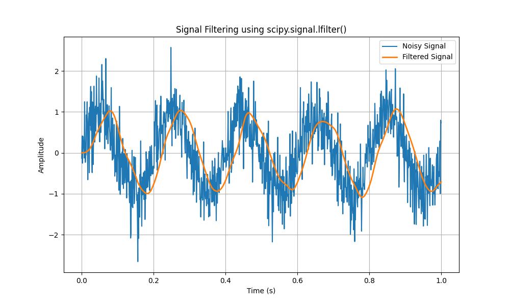
Filtering a Signal

Filtering is a crucial step in signal processing used to remove unwanted noise and extract useful information from signals. The scipy.signal.lfilter() function can be used to apply FIR or IIR filters to a signal efficiently.

Here is an example of filtering a noisy signal using a low-pass FIR filter and the scipy.signal.lfilter() function −

import numpy as np
from scipy.signal import lfilter, firwin
import matplotlib.pyplot as plt

# Generate a noisy signal
fs = 1000  # Sampling frequency
t = np.linspace(0, 1, fs, endpoint=False)  # Time vector
signal = np.sin(2 * np.pi * 5 * t) + 0.5 * np.random.randn(t.size)

# Design a low-pass FIR filter
numtaps = 51
cutoff = 10  # Cutoff frequency in Hz
b = firwin(numtaps, cutoff, fs=fs)

# Apply the filter
filtered_signal = lfilter(b, [1.0], signal)

# Plot the original and filtered signals
plt.figure(figsize=(10, 6))
plt.plot(t, signal, label='Noisy Signal')
plt.plot(t, filtered_signal, label='Filtered Signal', linewidth=2)
plt.title('Signal Filtering using scipy.signal.lfilter()')
plt.xlabel('Time (s)')
plt.ylabel('Amplitude')
plt.legend()
plt.grid()
plt.show()

Below is the output of filtering out high-frequency noise from a signal −

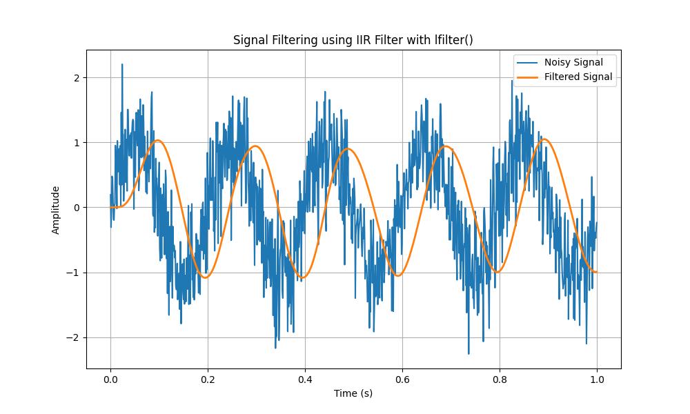
Applying an IIR Filter

Infinite Impulse Response (IIR) filters are widely used in signal processing due to their efficiency in achieving sharp frequency responses with fewer coefficients compared to FIR filters. The scipy.signal.lfilter() function allows the implementation of IIR filters by specifying the filter coefficients.

Here is an example of applying a Butterworth low-pass IIR filter using the scipy.signal.lfilter() function −

import numpy as np
from scipy.signal import butter, lfilter
import matplotlib.pyplot as plt

# Generate a noisy signal
fs = 1000  # Sampling frequency in Hz
t = np.linspace(0, 1, fs, endpoint=False)  # Time vector
signal = np.sin(2 * np.pi * 5 * t) + 0.5 * np.random.randn(t.size)

# Design a Butterworth low-pass filter
order = 4
cutoff = 10  # Cutoff frequency in Hz
b, a = butter(order, cutoff, fs=fs, btype='low')

# Apply the IIR filter
filtered_signal = lfilter(b, a, signal)

# Plot the original and filtered signals
plt.figure(figsize=(10, 6))
plt.plot(t, signal, label='Noisy Signal')
plt.plot(t, filtered_signal, label='Filtered Signal', linewidth=2)
plt.title('Signal Filtering using IIR Filter with lfilter()')
plt.xlabel('Time (s)')
plt.ylabel('Amplitude')
plt.legend()
plt.grid()
plt.show()

Following is the output of the IIR filter to remove high-frequency noise from a signal effectively −

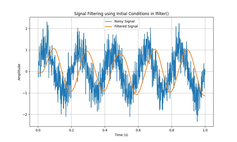
Filter with Initial Conditions

In some applications, it is important to maintain continuity when filtering segmented signals. The scipy.signal.lfilter() function provides the zi parameter which allows the specification of initial filter conditions to ensure a smooth transition between segments.

The zf variable contains the final filter conditions which can be used for further processing if the signal is segmented.

The initial conditions help to minimize filter startup transients and can be computed using the scipy.signal.lfilter_zi() function. Here is an example of applying a filter with initial conditions −

import numpy as np
from scipy.signal import butter, lfilter, lfilter_zi
import matplotlib.pyplot as plt

# Generate a noisy signal
fs = 1000  # Sampling frequency in Hz
t = np.linspace(0, 1, fs, endpoint=False)  # Time vector
signal = np.sin(2 * np.pi * 5 * t) + 0.5 * np.random.randn(t.size)

# Design a Butterworth low-pass filter
order = 4
cutoff = 10  # Cutoff frequency in Hz
b, a = butter(order, cutoff, fs=fs, btype='low')

# Compute initial conditions to start filter in steady state
zi = lfilter_zi(b, a) * signal[0]

# Apply the filter with initial conditions
filtered_signal, zf = lfilter(b, a, signal, zi=zi)

# Plot the original and filtered signals
plt.figure(figsize=(10, 6))
plt.plot(t, signal, label='Noisy Signal')
plt.plot(t, filtered_signal, label='Filtered Signal', linewidth=2)
plt.title('Signal Filtering using Initial Conditions in lfilter()')
plt.xlabel('Time (s)')
plt.ylabel('Amplitude')
plt.legend()
plt.grid()
plt.show()

Here is the output of the initial filter conditions help to start the filtering process without introducing transients by ensuring a more stable filtered output.