SciPy optimize.least_squares() Function

---

---

scipy.optimize.least_squares() function is a SciPy function for solving nonlinear least-squares optimization problems. It minimizes the sum of squares of residuals F(x) = f(x)2 where f(x) is a vector-valued function.

This function supports bounds on variables, robust loss functions and three solvers such as 'trf' (Trust Region Reflective), 'dogbox', and 'lm' (Levenberg-Marquardt). It is highly customizable, with options for Jacobian calculation, finite-difference approximations and solver-specific parameters.

The output includes the optimized parameters, residuals, cost and diagnostic information. It is widely used in curve fitting, parameter estimation and inverse problems.

Syntax

Following is the syntax of the function scipy.optimize.least_squares() which is used to solve nonlinear least-squares optimization problems −

least_squares(fun, x0, jac='2-point', bounds=(-inf, inf), method='trf', ftol=1e-08, xtol=1e-08, gtol=1e-08, x_scale=1.0, loss='linear', f_scale=1.0, diff_step=None, tr_solver=None, tr_options={}, jac_sparsity=None, max_nfev=None, verbose=0, args=(), kwargs={})

Parameters

Here are the parameters of the function scipy.optimize.least_squares() −

• fun(callable): The objective function to minimize. It should take an array x and return an array of residuals.
• x0(array_like): Initial guess for the parameters to optimize.
• jac(callable or str, optional): The Jacobian matrix of fun with respect to x. If callable then it should return an array of derivatives, if strings '2-point', '3-point' or 'cs' specify numerical approximation methods.
• bounds(tuple of array_like, optional): Lower and upper bounds for variables as (lb, ub).
• method(str, optional): This is the algorithm to use, which can be trf, dogbox and lm.
• ftol, xtol, gtol(float, optional): Tolerances for termination based on changes in cost function, parameter values or gradient norm, respectively.
• max_nfev (int, optional): Maximum number of function evaluations.
• diff_step (float or array_like, optional): Step size for numerical differentiation.
• tr_solver (str, optional): Solver for the trust-region problem such as 'exact' or 'lsmr'.
• loss (str or callable, optional): Loss function to reduce the sensitivity to outliers. The options for loss are 'linear', 'soft_l1', 'huber', 'cauchy', 'arctan'.
• f_scale (float, optional): Scale parameter for robust loss functions.
• verbose (int, optional): Level of verbosity (0 = silent, 1 = summary, 2 = progress).
• args (tuple, optional): Extra arguments to pass to fun.
• kwargs (dict, optional): Extra keyword arguments to pass to fun.

Return Value

scipy.optimize.least_squares() returns an OptimizeResult object.

Fitting an Exponential Decay Model

Following is the example which shows how to use the function scipy.optimize.least_squares() for minimizing residuals between observed data and a model y=ae^bt −

import numpy as np
from scipy.optimize import least_squares

# Residuals function
def residuals(x, t, y):
    return y - x[0] * np.exp(-x[1] * t)

# Data
t_data = np.linspace(0, 10, 100)
y_data = 3 * np.exp(-1.5 * t_data) + 0.1 * np.random.randn(100)

# Initial guess
x0 = [1, 0.1]

# Solve
result = least_squares(residuals, x0, args=(t_data, y_data))
print("Optimal parameters:", result.x)
print("Final cost:", result.cost)

Here is the output of the scipy.optimize.least_squares() function for minimizing resuidals −

Final cost: 0.5337646918947744

Solving a Simple Linear System

Heres an example of solving a simple linear system using scipy.optimize.least_squares(). Let's consider solving the linear system Ax=b in a least-squares sense where A is a given matrix and b is the target vector −

import numpy as np
from scipy.optimize import least_squares

# Define the problem
A = np.array([[2, 1], [1, 3]])
b = np.array([8, 13])

# Define the residual function
def residuals(x):
    return A @ x - b

# Initial guess
x0 = np.zeros(A.shape[1])

# Solve the least squares problem
result = least_squares(residuals, x0)

# Display the results
print("Solution x:", result.x)
print("Residual norm:", result.cost)
print("Residuals:", result.fun)

Here is the output of the scipy.optimize.least_squares() function which is used for solving a simple linear system −

Solution x: [2.2 3.6]
Residual norm: 6.310887241768095e-30
Residuals: [ 0.00000000e+00 -3.55271368e-15]

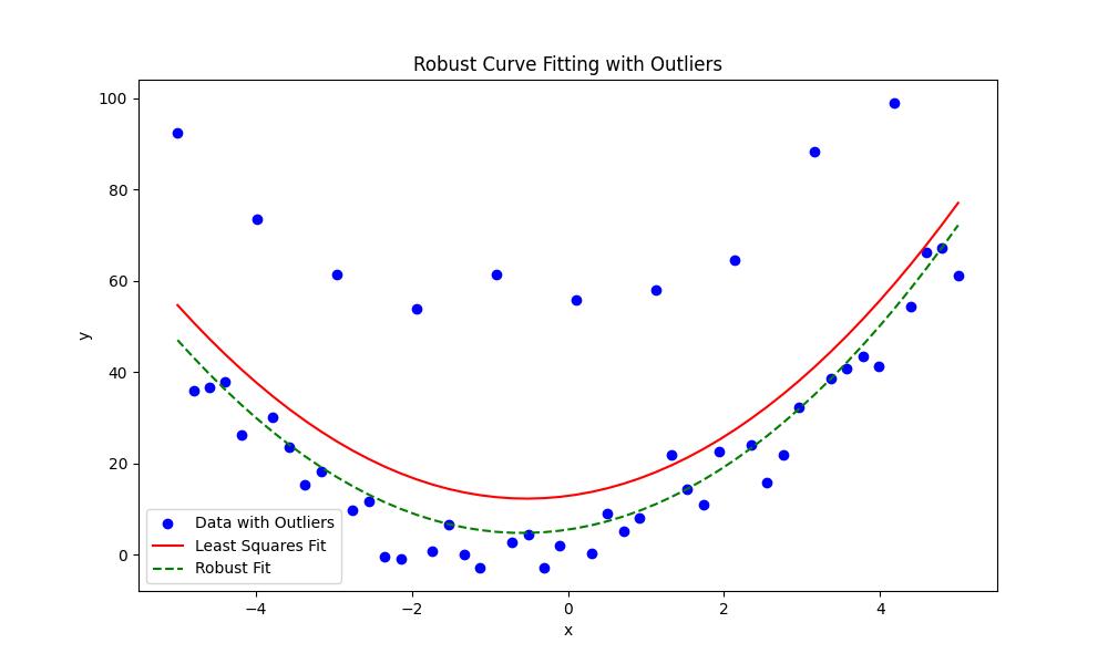
Robust Curve Fitting with Outliers

When fitting a curve to data with outliers, robust methods reduce the impact of outliers on the fit. scipy.optimize.least_squares() supports robust loss functions by making it suitable for such scenarios. Here in this example we fit a quadratic curve ax²+bx+c to data with outliers − −

import numpy as np
import matplotlib.pyplot as plt
from scipy.optimize import least_squares

# Generate synthetic data
np.random.seed(42)
x = np.linspace(-5, 5, 50)
y = 2 * x**2 + 3 * x + 5 + np.random.normal(scale=5, size=x.shape)

# Introduce outliers
y[::5] += 50  # Adding large outliers every 5th point

# Define the model
def model(params, x):
    a, b, c = params
    return a * x**2 + b * x + c

# Define the residual function
def residuals(params, x, y):
    return model(params, x) - y

# Initial guess
initial_params = [1, 1, 1]

# Fit without robust loss
result_no_robust = least_squares(residuals, initial_params, args=(x, y))

# Fit with robust loss
result_robust = least_squares(
    residuals, initial_params, args=(x, y), loss='soft_l1', f_scale=10
)

# Plot the results
plt.figure(figsize=(10, 6))
plt.scatter(x, y, label="Data with Outliers", color="blue")
plt.plot(x, model(result_no_robust.x, x), label="Least Squares Fit", color="red")
plt.plot(x, model(result_robust.x, x), label="Robust Fit", color="green", linestyle="--")
plt.legend()
plt.xlabel("x")
plt.ylabel("y")
plt.title("Robust Curve Fitting with Outliers")
plt.show()

Here is the output of the scipy.optimize.least_squares() function which is used for solving a simple linear system −

Solution x: [2.2 3.6]
Residual norm: 6.310887241768095e-30
Residuals: [ 0.00000000e+00 -3.55271368e-15]

Here is the output of the robust curve fitting with outliers −