SciPy Optimize.curve_fit() Function

---

---

scipy.optimize.curve_fit() is a function in SciPy used to fit a curve to a set of data points by optimizing the parameters of a given model. It uses non-linear least squares to minimize the difference between the observed data and the values predicted by the model function.

This function takes the model, independent variable data, dependent variable data and initial parameter estimates as input. It returns the optimal parameter values and the covariance matrix which provides the uncertainty of the estimates. This function is widely used for curve fitting tasks such as linear, polynomial and custom non-linear models.

Syntax

Following is the syntax of using the scipy.optimize.curve_fit() function −

curve_fit(f, xdata, ydata, p0=None, sigma=None, absolute_sigma=False, check_finite=None, bounds=(-inf, inf), method=None, jac=None, *, full_output=False, nan_policy=None, **kwargs)

Below are the parameters of the scipy.optimize.curve_fit() function −

• f: This the model function to be fitted. This should take the independent variable as the first argument and the parameters to be optimized as subsequent arguments.
• xdata(array-like): The independent variable data. If our data is multi-dimensional then xdata must be a tuple.
• ydata(array-like): The dependent variable data that we want to fit. Must be of the same length as xdata.
• p0(optional): Initial guess for the parameters. It should be an array of the same length as the number of parameters in f. Defaults to 1 for all parameters if not provided.
• sigma(optional): Standard deviation of ydata. If provided then this is used as weights in the fitting process. If absolute_sigma is False then it is relative weights; if True then the weights are absolute values.
• absolute_sigma (optional): Default value is False. If True then the sigma is taken as absolute standard deviations of ydata, otherwise it is relative.
• check_finite (optional): Default value is True. If True then it checks whether the input arrays contain any infinities or NaNs. Disabling may improve performance.
• bounds(optional): Bounds for the parameters if provided as a tuple of two arrays as ([lower_bounds], [upper_bounds]). Each element represents the bounds for a particular parameter. By default bounds are set to (-inf, inf) for each parameter i.e., no bounds.
• method(optional): This specifies the optimization method. The default value is lm (Levenberg-Marquardt) which doesnt support bounds. If bounds are used then trf (Trust Region Reflective) or dogbox can be chosen.
• jac(optional): The Jacobian matrix of the model with respect to the parameters. Only used when method is not lm.
• full_output(optional): Default value is False. If True then the additional information is returned as part of the output such as convergence information and diagnostic messages.
• nan_policy(optional): Determines how to handle NaN values in the data. Options are such as propagate, omit,raise.
• kwargs: Additional arguments passed to the underlying optimizer depending on the method chosen.

Return Value

The scipy.optimize.curve_fit() function returns two main outputs one is optimal parameters(popt) and covariance matrix(pcov).

Example 1

Following is the example of performing a linear fit using the scipy.optimize.curve_fit() function in Python. The goal is to fit a line = + to a given set of data points −

import numpy as np
from scipy.optimize import curve_fit
import matplotlib.pyplot as plt

# Example data
x_data = np.array([0, 1, 2, 3, 4, 5])
y_data = np.array([2.1, 2.9, 3.7, 4.6, 5.1, 6.2])

# Define a linear model: y = ax + b
def linear_model(x, a, b):
    return a * x + b

# Perform curve fitting
params, covariance = curve_fit(linear_model, x_data, y_data)

# Extract the fitted parameters (a = slope, b = intercept)
a_fit, b_fit = params
print(f"Fitted parameters: a = {a_fit:.2f}, b = {b_fit:.2f}")

# Plot the original data points
plt.scatter(x_data, y_data, label="Data", color="blue")

# Plot the fitted line using the optimized parameters
plt.plot(x_data, linear_model(x_data, a_fit, b_fit), label=f"Fitted line: y = {a_fit:.2f}x + {b_fit:.2f}", color="red")

# Add labels and legend
plt.xlabel("x")
plt.ylabel("y")
plt.title("Linear Fit Example")
plt.legend()

# Display the plot
plt.show()

Below is the output of the scipy.optimize.curve_fit() function which is used to perform linear curve fitting −

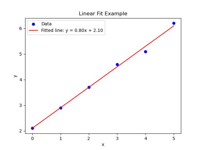
Fitted parameters: a = 0.80, b = 2.10

Example 2

Here is the example of using the function scipy.optimize.curve_fit() which is used for non-linear fit of an exponential function. The exponential model here we are using is = + −

import numpy as np
from scipy.optimize import curve_fit
import matplotlib.pyplot as plt

# Example data
x_data = np.array([0, 1, 2, 3, 4, 5])
y_data = np.array([2.1, 2.9, 3.7, 4.6, 5.1, 6.2])

# Define a linear model: y = ax + b
def linear_model(x, a, b):
    return a * x + b

# Perform curve fitting
params, covariance = curve_fit(linear_model, x_data, y_data)

# Extract the fitted parameters (a = slope, b = intercept)
a_fit, b_fit = params
print(f"Fitted parameters: a = {a_fit:.2f}, b = {b_fit:.2f}")

# Plot the original data points
plt.scatter(x_data, y_data, label="Data", color="blue")

# Plot the fitted line using the optimized parameters
plt.plot(x_data, linear_model(x_data, a_fit, b_fit), label=f"Fitted line: y = {a_fit:.2f}x + {b_fit:.2f}", color="red")

# Add labels and legend
plt.xlabel("x")
plt.ylabel("y")
plt.title("Linear Fit Example")
plt.legend()

# Display the plot
plt.show()

Following is the output of the scipy.optimize.curve_fit() function which is used to perform Exponential curve fitting −

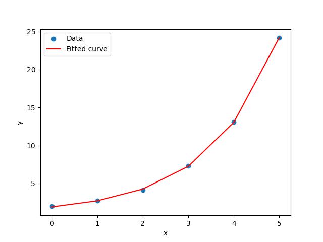
Fitted parameters: a = 0.8614775300447255, b = 0.658438935283945, c = 1.0461615515030036

Example 3

In this example we are using the function scipy.optimize.curve_fit() which is used for fitting a polynomial curve specifically a quadratic polynomial = ²++ to a set of data points −

import numpy as np
from scipy.optimize import curve_fit
import matplotlib.pyplot as plt

# Example data: x and corresponding y values
x_data = np.array([0, 1, 2, 3, 4, 5])
y_data = np.array([1, 1.8, 3.5, 6.2, 10.1, 15])

# Define the quadratic model y = ax^2 + bx + c
def quadratic_model(x, a, b, c):
    return a * x**2 + b * x + c

# Use curve_fit to find the optimal parameters a, b, and c
params, covariance = curve_fit(quadratic_model, x_data, y_data)

# Extract fitted parameters
a_fit, b_fit, c_fit = params
print(f"Fitted parameters: a = {a_fit}, b = {b_fit}, c = {c_fit}")

# Plot the original data
plt.scatter(x_data, y_data, label="Data", color="blue")

# Plot the fitted quadratic curve
x_fit = np.linspace(0, 5, 100)  # Create smooth x values for plotting the curve
y_fit = quadratic_model(x_fit, a_fit, b_fit, c_fit)
plt.plot(x_fit, y_fit, label="Fitted Curve", color="red")

# Customize and show the plot
plt.legend()
plt.xlabel("x")
plt.ylabel("y")
plt.title("Polynomial Fit (Quadratic)")
plt.grid(True)
plt.show()

Below is the output of the scipy.optimize.curve_fit() function which is used to perform Polynomial curve fitting −

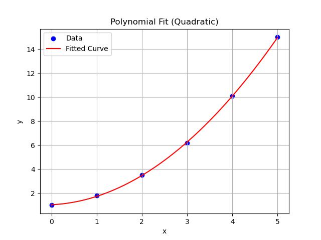
Fitted parameters: a = 0.5232142857132461, b = 0.17249999999819343, c = 1.0392857142858025