SciPy - ndimage.grey_opening() Function

---

---

The scipy.ndimage.grey_opening() is a function in the scipy.ndimage module, which is used to perform grey-level morphological opening on an image. It applies an erosion followed by a dilation operation using a specific structuring element.

The purpose of grey-level opening is to remove small objects or noise from an image while preserving the shape and size of larger structures.

Unlike binary opening which works on binary images where grey-level opening operates on grayscale images by preserving the intensity of pixels. This function requires an input image and a structuring element to define the neighborhood used in the operation.

Syntax

Following is the syntax of the function scipy.ndimage.grey_opening() to perform grey scale Opening operation on the input image −

scipy.ndimage.grey_opening(input, size=None, footprint=None, structure=None, output=None, mode='reflect', cval=0.0, origin=0, *, axes=None)

Parameters

Following are the parameters of the scipy.ndimage.grey_opening() function −

• input: The input image or array on which the grayscale opening operation is applied. It can be a binary or grayscale image.
• size (optional): The size of the structuring element used for the opening operation and specified as a tuple e.g., (3, 3). This defines the neighborhood dimensions.
• footprint (optional): A binary array that defines the shape of the structuring element. It overrides the size parameter when provided.
• structure (optional): An array specifying the weights for the structuring element. It overrides both size and footprint if provided.
• output (optional): The array where the result of the operation is stored. If not specified then a new array is created.
• mode (optional): This parameter defines how the boundaries of the image are handled and the available modes are 'reflect', 'constant', 'nearest', 'mirror' and 'wrap'. The default value is 'reflect'.
• cval (optional): The constant value used for padding when mode='constant'. The default value is 0.0.
• origin (optional): It controls the placement of the structuring element relative to the current pixel. A value of 0 centers the element and positive or negative values shift it.

Return Value

The scipy.ndimage.grey_opening() function returns the processed array after applying the grayscale morphological opening.

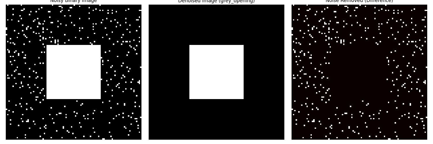
Noise Removal in a Binary Image

Grayscale morphological operations are powerful techniques for image preprocessing. One common application of grayscale opening grey_opening() is to remove small noise or unwanted details in a binary image while preserving the overall structure. Following is the example which shows how to use grey_opening() function to remove noise −

import numpy as np
import scipy.ndimage as ndi
import matplotlib.pyplot as plt

# Create a noisy binary image (100x100 pixels)
np.random.seed(42)  # For reproducibility
binary_image = np.zeros((100, 100), dtype=int)
binary_image[30:70, 30:70] = 1  # Main object (square)
noise = np.random.random((100, 100)) > 0.95  # Random noise
noisy_image = binary_image | noise  # Combine object and noise

# Apply grey_opening to remove noise
denoised_image = ndi.grey_opening(noisy_image, size=(3, 3))

# Display the original and processed images
fig, axes = plt.subplots(1, 3, figsize=(15, 5))

# Original binary image with noise
axes[0].imshow(noisy_image, cmap='gray')
axes[0].set_title("Noisy Binary Image")
axes[0].axis("off")

# Denoised binary image
axes[1].imshow(denoised_image, cmap='gray')
axes[1].set_title("Denoised Image (grey_opening)")
axes[1].axis("off")

# Highlight difference
difference = noisy_image ^ denoised_image
axes[2].imshow(difference, cmap='hot')
axes[2].set_title("Noise Removed (Difference)")
axes[2].axis("off")

plt.tight_layout()
plt.show()

Here is the output of the function scipy.ndimage.grey_opening() which is used to implement Greyscale opening to remove noise −

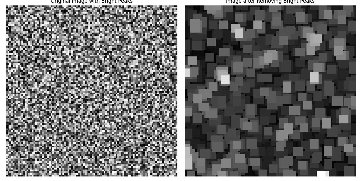
Removing Bright Peaks

In image processing, bright peaks are small regions of high intensity that can appear due to noise or artifacts. These peaks can distort analysis or visualization. Morphological grayscale opening is a common technique to remove such bright peaks while preserving larger structures in the image. The grey_opening() function from scipy.ndimage achieves this by applying erosion followed by dilation using a structuring element. Below is the example of using the function scipy.ndimage.grey_opening() for removing the bright peas from an image −

import numpy as np
import scipy.ndimage as ndi
import matplotlib.pyplot as plt

# Create a synthetic grayscale image (100x100 pixels)
np.random.seed(42)  # For reproducibility
image = np.random.random((100, 100))  # Random grayscale values between 0 and 1

# Add bright peaks to the image
image[20, 30] = 1.0
image[50, 50] = 1.0
image[70, 80] = 1.0

# Apply grey_opening to remove bright peaks
size = (5, 5)  # Structuring element size
processed_image = ndi.grey_opening(image, size=size)

# Display the original and processed images
fig, axes = plt.subplots(1, 2, figsize=(12, 6))

# Original image
axes[0].imshow(image, cmap='gray')
axes[0].set_title("Original Image with Bright Peaks")
axes[0].axis("off")

# Processed image
axes[1].imshow(processed_image, cmap='gray')
axes[1].set_title("Image after Removing Bright Peaks")
axes[1].axis("off")

plt.tight_layout()
plt.show()

Here is the output of the function scipy.ndimage.grey_opening() which is used to implement Greyscale opening to remove bright peaks −

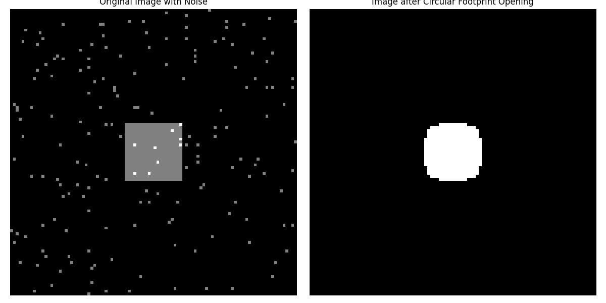
Handling Non-Rectangular Neighborhoods with Footprint

While rectangular structuring elements are common in morphological operations which are certain applications require non-rectangular neighborhoods for more flexible processing. The footprint parameter in grey_opening() or similar functions in scipy.ndimage let us define custom-shaped structuring elements such as circles, crosses or other shapes for more precise control over the operation. Here is the example of showing how to use the scipy.ndimage.grey_opening() function for handling non-rectangular neighborhoods i.e., circular footprint with footprint −

import numpy as np
import scipy.ndimage as ndi
import matplotlib.pyplot as plt

# Create a synthetic grayscale image (100x100 pixels)
np.random.seed(42)
image = np.zeros((100, 100), dtype=float)
image[40:60, 40:60] = 1  # Square object
noise = np.random.random((100, 100)) > 0.98  # Add random noise
image = image + noise  # Combine object and noise

# Create a circular footprint
radius = 5
y, x = np.ogrid[-radius:radius+1, -radius:radius+1]
footprint = x**2 + y**2 <= radius**2

# Apply grey_opening with a circular footprint
processed_image = ndi.grey_opening(image, footprint=footprint)

# Display the original and processed images
fig, axes = plt.subplots(1, 2, figsize=(12, 6))

# Original image
axes[0].imshow(image, cmap='gray')
axes[0].set_title("Original Image with Noise")
axes[0].axis("off")

# Processed image
axes[1].imshow(processed_image, cmap='gray')
axes[1].set_title("Image after Circular Footprint Opening")
axes[1].axis("off")

plt.tight_layout()
plt.show()

Here is the output of the function scipy.ndimage.grey_opening() which is used to implement Greyscale opening to handle Non Rectangular Neighborhoods with footprints −