SciPy - ndimage.binary_opening() Function

---

---

The scipy.ndimage.binary_opening() is a function in SciPy. This perform a morphological operation, which is used to remove small objects from a binary image. It combines two operations erosion followed by dilation.

The erosion step shrinks the boundaries of the foreground (1s) and the dilation step expands the eroded image back to its original size but without the smaller objects that were eroded.

This operation is useful for noise removal, separating connected components and smoothing contours in binary images. The size and shape of the structuring element can be customized and the process can be repeated using the iterations parameter.

Syntax

Following is the syntax of the function scipy.ndimage.binary_opening() to perform Opening morphological operation on an image −

scipy.ndimage.binary_opening(input, structure=None, iterations=1, output=None, origin=0, mask=None, border_value=0, brute_force=False)[source]

Parameters

Following are the parameters of the scipy.ndimage.binary_opening() function −

• input: The input image or array which can be binary or grayscale, on which the binary opening operation is applied.
• structure(optional): It is an array that explicitly specifies the structuring element. By default a cross-shaped structuring element is used.
• iterations(optional): The number of times the opening operation is applied. By default, it is set to 1. If set to -1 then the opening operation is applied until the result no longer changes.
• mask(optional): A binary mask that limits the opening operation to specific areas of the input image and only regions where the mask is non-zero will be processed.
• output(optional): This is an array where the result will be stored. If not provided then a new array is allocated.
• border_value(optional): This parameter specifies the value used for padding the borders of the image. It can be 0 or 1 with a default value of 0.
• origin(optional): This parameter controls the placement of the structuring element relative to the current pixel. A value of 0 centers the structuring element at the pixel. Positive or negative values shift the structuring element.
• brute_force(optional): If True then a brute-force method is used for the opening operation which can be slower but may handle certain custom structuring elements more effectively. The default value is False.

Return Value

The scipy.ndimage.binary_opening() function returns a binary array that represents the result of applying the binary opening operation on the input image.

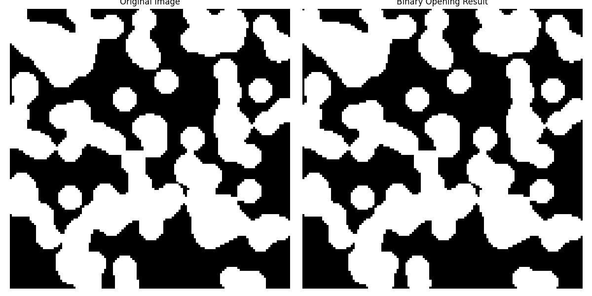
Example of Basic Binary Opening

Following is the example of the function scipy.ndimage.binary_opening() in which the binary opening operation is applied using the default structuring element i.e., cross-shaped and a single iteration −

import numpy as np
import matplotlib.pyplot as plt
from skimage.data import binary_blobs
from scipy.ndimage import binary_opening

# Generate a sample binary image
image = binary_blobs(length=128, blob_size_fraction=0.1)

# Apply binary opening with the default parameters (cross-shaped structuring element)
result = binary_opening(image)

# Plot the original and opened images
plt.figure(figsize=(12, 6))

plt.subplot(1, 2, 1)
plt.title("Original Image")
plt.imshow(image, cmap='gray')
plt.axis('off')

plt.subplot(1, 2, 2)
plt.title("Binary Opening Result")
plt.imshow(result, cmap='gray')
plt.axis('off')

plt.tight_layout()
plt.show()

Here is the output of the function scipy.ndimage.binary_opening() which is used to implement basic Example of Binary Opening −

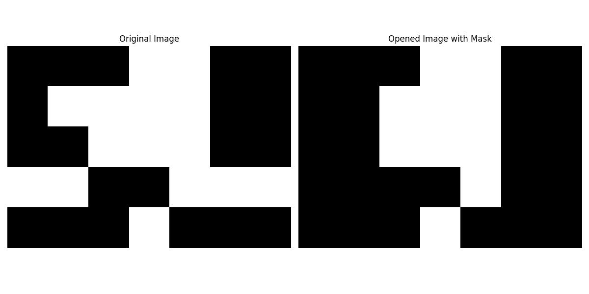
Binary Opening with Masking

When combined masking and binary opening applied selectively to specific regions of an image then the mask defines the areas of the image where the operation should be performed, while areas outside the mask remain unchanged. Here in this example we'll show how to perform binary opening with a mask using scipy.ndimage.binary_opening() −

import numpy as np
import matplotlib.pyplot as plt
from scipy.ndimage import binary_opening

# Create a binary image (with some small noise)
binary_image = np.array([[0, 0, 0, 1, 1, 0, 0],
                         [0, 1, 1, 1, 1, 0, 0],
                         [0, 0, 1, 1, 1, 0, 0],
                         [1, 1, 0, 0, 1, 1, 1],
                         [0, 0, 0, 1, 0, 0, 0]])

# Create a binary mask to limit the opening to specific regions
mask = np.array([[0, 0, 0, 1, 1, 0, 0],
                 [0, 1, 1, 1, 0, 0, 0],
                 [0, 0, 1, 0, 0, 0, 0],
                 [1, 1, 0, 0, 1, 1, 1],
                 [0, 0, 0, 0, 0, 0, 0]])

# Apply binary opening with the mask
opened_image = binary_opening(binary_image, mask=mask)

# Display the original and the opened image
plt.figure(figsize=(12, 6))

# Original Image
plt.subplot(1, 2, 1)
plt.title("Original Image")
plt.imshow(binary_image, cmap='gray', interpolation='nearest')
plt.axis('off')

# Opened Image with Mask
plt.subplot(1, 2, 2)
plt.title("Opened Image with Mask")
plt.imshow(opened_image, cmap='gray', interpolation='nearest')
plt.axis('off')

plt.tight_layout()
plt.show()

Here is the output of the function scipy.ndimage.binary_opening() which performed binary opening with masking −

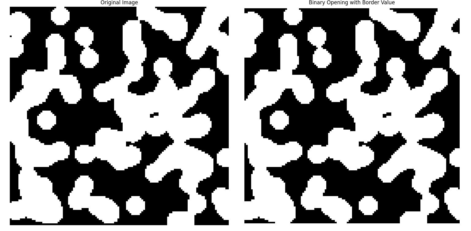
Binary Opening with Border Value

In some cases we may want to control how the operation handles the borders of the image. The border_value parameter in scipy.ndimage.binary_opening() controls how the borders of the image are treated. This example shows the effect of using a custom border value during binary opening applied in an image −

import numpy as np
import matplotlib.pyplot as plt
from scipy.ndimage import binary_opening
from skimage.data import binary_blobs

# Set the random seed for reproducibility
np.random.seed(1)

# Load a sample binary image
image = binary_blobs(length=128, blob_size_fraction=0.1)

# Apply binary opening with a border value of 1
result = binary_opening(image, border_value=1)

# Plot the original and opened images
plt.figure(figsize=(12, 6))

plt.subplot(1, 2, 1)
plt.title("Original Image")
plt.imshow(image, cmap='gray')
plt.axis('off')

plt.subplot(1, 2, 2)
plt.title("Binary Opening with Border Value")
plt.imshow(result, cmap='gray')
plt.axis('off')

plt.tight_layout()
plt.show()

Here is the output of the function scipy.ndimage.binary_opening() which performed binary opening with Border value −