SciPy - interpolate.RectBivariateSpline() Function

scipy.interpolate.RectBivariateSpline() is a function in the SciPy library which is used for smooth, two-dimensional interpolation over a rectangular grid. It constructs a bivariate spline that can efficiently interpolate values for data defined on a grid especially when smooth surface fitting is required.

When x and y coordinates and corresponding z values are passed to RectBivariateSpline() then it creates a continuous function to estimate values at arbitrary points within the grids bounds. This is ideal for smooth contour plotting, surface analysis or filling in missing grid data with control over smoothness via spline degrees and a smoothing factor for better fitting.

Syntax

Following is the syntax of the function scipy.interpolate.RectBivariateSpline() which is used to perform interpolation−

scipy.interpolate.RectBivariateSpline(x, y, z, bbox=[None, None, None, None], kx=3, ky=3, s=0)

Parameters

Following are the parameters of the scipy.interpolate.RectBivariateSpline() function −

• x(array-like, shape (m,)): The 1-dimensional array of x values where data points are located. This must be increasing.
• y(array-like, shape (n,)): The 1-dimensional array of y values where data points are located. This must be increasing.
• z(array-like, shape (m, n)): The 2-dimensional array of z values which are dependent values at grid points. Each value in z corresponds to a (x, y) pair.
• bbox(list, optional): This parameter specifies the bounding box [xmin, xmax, ymin, ymax] for the interpolated data. The default value to the range of x and y.
• kx(int, optional): This parameter is the degree of the spline in the x direction. Default value is 3 which means a cubic spline.
• ky(int, optional): This is the degree of the spline in the y direction. Default value is 3.
• s(float, optional): This is the smoothing factor. Default value is 0 for no smoothing (interpolation). A higher value will result in a smoother fit.

Return Value

The scipy.interpolate.RectBivariateSpline() function returns a spline object that can be used to interpolate values at new (x, y) coordinates.

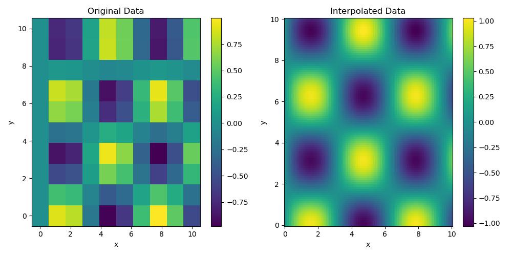
Basic Interpolation on a Grid

Following is the example of scipy.interpolate.RectBivariateSpline() function in which we are setting up a grid of x and y values by defining a function over that grid and interpolate values between grid points −

import numpy as np
from scipy.interpolate import RectBivariateSpline
import matplotlib.pyplot as plt

# Step 1: Define a grid of x and y values
x = np.linspace(0, 10, 10)  # 10 points from 0 to 10 on x-axis
y = np.linspace(0, 10, 10)  # 10 points from 0 to 10 on y-axis
X, Y = np.meshgrid(x, y)    # Create a 2D grid from x and y

# Step 2: Define some function over this grid (e.g., Z = sin(x) * cos(y))
Z = np.sin(X) * np.cos(Y)

# Step 3: Create the bivariate spline interpolator
spline = RectBivariateSpline(x, y, Z)

# Step 4: Define a denser grid for interpolation
x_new = np.linspace(0, 10, 100)  # 100 points from 0 to 10 on x-axis
y_new = np.linspace(0, 10, 100)  # 100 points from 0 to 10 on y-axis

# Interpolate Z values on the new grid
Z_new = spline(x_new, y_new)

# Step 5: Plot the original and interpolated data
plt.figure(figsize=(10, 5))

# Plot the original data
plt.subplot(1, 2, 1)
plt.title("Original Data")
plt.pcolormesh(X, Y, Z, shading='auto', cmap='viridis')
plt.colorbar()
plt.xlabel("x")
plt.ylabel("y")

# Plot the interpolated data
plt.subplot(1, 2, 2)
plt.title("Interpolated Data")
plt.pcolormesh(np.meshgrid(x_new, y_new)[0], np.meshgrid(x_new, y_new)[1], Z_new, shading='auto', cmap='viridis')
plt.colorbar()
plt.xlabel("x")
plt.ylabel("y")

plt.tight_layout()
plt.show()

Here is the output of the scipy.interpolate.RectBivariateSpline() function which is used for basic interpolation on a grid −

Interpolation at Specific Points

In this example to interpolate at specific points using RectBivariateSpline() we can simply call the spline object with the desired x and y values and set grid=False. This allows us to get interpolated values at arbitrary points without creating a new mesh grid −

import numpy as np
from scipy.interpolate import RectBivariateSpline

# Define a grid of x and y values
x = np.linspace(0, 10, 10)  # 10 points from 0 to 10 on x-axis
y = np.linspace(0, 10, 10)  # 10 points from 0 to 10 on y-axis
X, Y = np.meshgrid(x, y)

# Define some function values over this grid (e.g., Z = sin(x) * cos(y))
Z = np.sin(X) * np.cos(Y)

# Create the bivariate spline interpolator
spline = RectBivariateSpline(x, y, Z)

# Define specific points where you want to interpolate
x_points = [1.5, 4.5, 7.5]
y_points = [2.5, 5.5, 8.5]

# Interpolate at these specific points
interpolated_values = spline(x_points, y_points, grid=False)

# Print the interpolated values at the specified points
for (xp, yp, value) in zip(x_points, y_points, interpolated_values):
    print(f"Interpolated value at (x={xp}, y={yp}): {value}")

Following is the output of the scipy.interpolate.RectBivariateSpline() function which is used to interpolate at specific points −

Interpolated value at (x=1.5, y=2.5): 0.03976979895549303
Interpolated value at (x=4.5, y=5.5): 0.1489405339121976
Interpolated value at (x=7.5, y=8.5): 0.2690972563333087

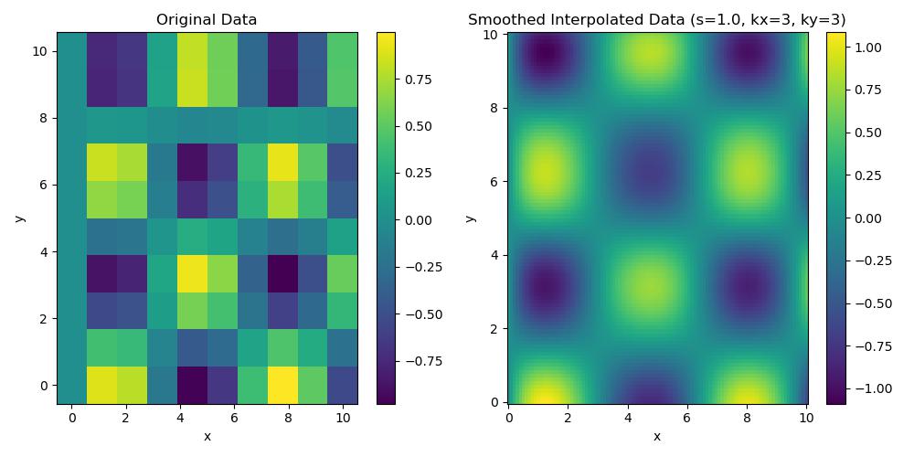
Using Different Degrees and Smoothing

In RectBivariateSpline() function we can control the smoothness and flexibility of the interpolation by adjusting the degrees of the spline by using kx and ky for the x and y axes and applying a smoothing factor i.e., s −

import numpy as np
from scipy.interpolate import RectBivariateSpline
import matplotlib.pyplot as plt

# Define a grid of x and y values
x = np.linspace(0, 10, 10)  # 10 points on the x-axis
y = np.linspace(0, 10, 10)  # 10 points on the y-axis
X, Y = np.meshgrid(x, y)

# Define function values on this grid (e.g., Z = sin(x) * cos(y))
Z = np.sin(X) * np.cos(Y)

# Create a bivariate spline interpolator with smoothing and different degrees
# kx=3, ky=3 implies cubic splines for both x and y; s=1.0 applies a moderate smoothing
spline = RectBivariateSpline(x, y, Z, kx=3, ky=3, s=1.0)

# Define a finer grid for interpolation
x_new = np.linspace(0, 10, 100)  # 100 points on the x-axis
y_new = np.linspace(0, 10, 100)  # 100 points on the y-axis

# Interpolate on the new grid
Z_new = spline(x_new, y_new)

# Plot original and smoothed interpolated data
plt.figure(figsize=(10, 5))

# Original data plot
plt.subplot(1, 2, 1)
plt.title("Original Data")
plt.pcolormesh(X, Y, Z, shading='auto', cmap='viridis')
plt.colorbar()
plt.xlabel("x")
plt.ylabel("y")

# Interpolated data with smoothing
plt.subplot(1, 2, 2)
plt.title("Smoothed Interpolated Data (s=1.0, kx=3, ky=3)")
plt.pcolormesh(np.meshgrid(x_new, y_new)[0], np.meshgrid(x_new, y_new)[1], Z_new, shading='auto', cmap='viridis')
plt.colorbar()
plt.xlabel("x")
plt.ylabel("y")

plt.tight_layout()
plt.show()

Following is the output of the scipy.interpolate.RectBivariateSpline() function which is used at different degrees and smoothing −