SciPy - interpolate.Rbf() Function

scipy.interpolate.Rbf() is a function in SciPys interpolation module that performs radial basis function (RBF) interpolation. This is ideal for interpolating scattered and multidimensional data. It constructs an interpolating function based on RBFs like Gaussian, multiquadratic or inverse multiquadratic functions.

The users pass input data points and their values which Rbf fits by creating a smooth surface across these points. This resulting function can then predict values at new points in the domain. The prameters of Rbf() function control the RBF type, smoothness and weighting by offering flexibility for applications in multidimensional surface fitting, spatial data analysis and numerical modeling.

Syntax

Following is the syntax of the function scipy.interpolate.Rbf() which is used to perform radial basis function −

scipy.interpolate.Rbf(*args, function='multiquadric', epsilon=None, smooth=0, norm=None)

Parameters

Following are the parameters of the scipy.interpolate.Rbf() function −

• *args: This takes the coordinates and values of our data points.
• function : This specificies the RBF to use. The available functions are multiquadric, inverse, gaussian, linear, cubic, quintic and thin_plate. The default function is multiquadric.
• epsilon (optional): A scaling parameter for some of the RBF functions. The default value depends on the average distance between points.
• smooth: This is the smoothing factor which adjusts the interpolation smoothness. A value of 0 means exact interpolation.
• norm (optional): The distance metric to use. If not specified, it defaults to the Euclidean norm.

Return Value

The scipy.interpolate.Rbf() function returns an instance of a radial basis function (RBF) interpolator which allows us to perform multidimensional interpolation.

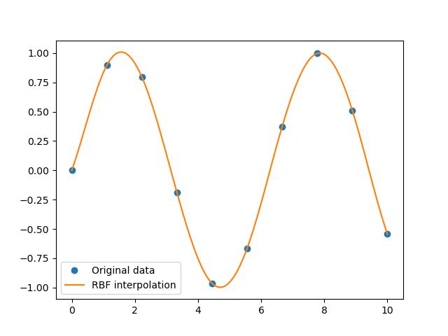
1D Interpolation

Following is the example of scipy.interpolate.Rbf() function. This example shows 1D interpolation where we have scattered points in one dimension and we use Rbf to interpolate between these points −

import numpy as np
import matplotlib.pyplot as plt
from scipy.interpolate import Rbf

# Sample data points
x = np.linspace(0, 10, 10)
y = np.sin(x)

# Create the RBF interpolator
rbf = Rbf(x, y, function='multiquadric')

# Interpolated points
x_interp = np.linspace(0, 10, 100)
y_interp = rbf(x_interp)

# Plot the result
plt.plot(x, y, 'o', label='Original data')
plt.plot(x_interp, y_interp, '-', label='RBF interpolation')
plt.legend()
plt.show()

Here is the output of the scipy.interpolate.Rbf() function used for 1d interpolation −

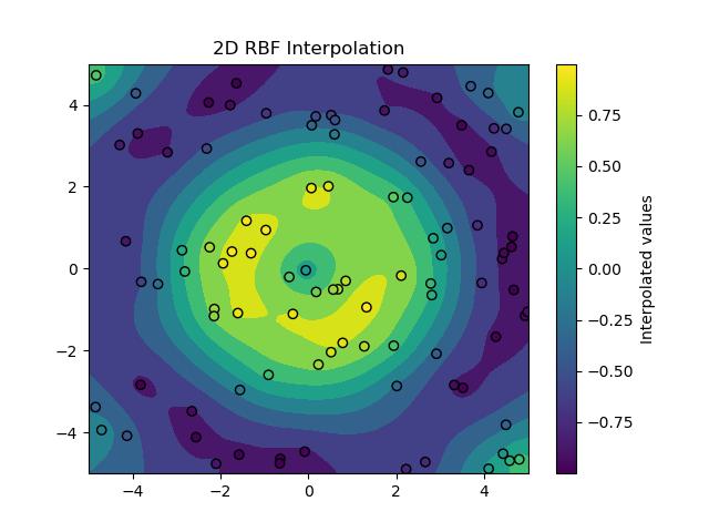
2D Interpolation

In this example we interpolate data in two dimensions. We define scattered points on a 2D grid and use Rbf to approximate values on a finer grid −

import numpy as np
import matplotlib.pyplot as plt
from scipy.interpolate import Rbf

# Create sample data points
x = np.random.uniform(-5, 5, 100)
y = np.random.uniform(-5, 5, 100)
z = np.sin(np.sqrt(x**2 + y**2))

# Create the RBF interpolator
rbf = Rbf(x, y, z, function='linear')

# Define grid for interpolation
xi = np.linspace(-5, 5, 100)
yi = np.linspace(-5, 5, 100)
xi, yi = np.meshgrid(xi, yi)
zi = rbf(xi, yi)

# Plot the result
plt.contourf(xi, yi, zi, cmap='viridis')
plt.scatter(x, y, c=z, cmap='viridis', edgecolor='k')
plt.colorbar(label='Interpolated values')
plt.title('2D RBF Interpolation')
plt.show()

Following is the output of the scipy.interpolate.Rbf() function which is used for 2d interpolation −

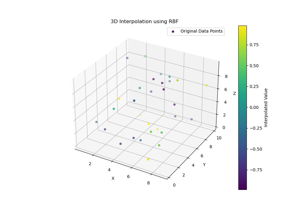
3D Interpolation

In 3D interpolation using scipy.interpolate.Rbf() function we can create an interpolating function for scattered data points in three-dimensional space. This is particularly useful when we have values measured at irregular spatial coordinates and want to predict values at other points. Here is the example of it −

import numpy as np
from scipy.interpolate import Rbf
from mpl_toolkits.mplot3d import Axes3D
import matplotlib.pyplot as plt

# Generate random 3D data points
x = np.random.uniform(0, 10, 30)  # Random x-coordinates
y = np.random.uniform(0, 10, 30)  # Random y-coordinates
z = np.random.uniform(0, 10, 30)  # Random z-coordinates

# Calculate values based on a known function (e.g., sine of the radial distance)
values = np.sin(np.sqrt(x**2 + y**2 + z**2))

# Create the RBF interpolator
rbf = Rbf(x, y, z, values, function='multiquadric', smooth=0.1)

# Create a 3D grid where we want to interpolate the values
xi, yi, zi = np.meshgrid(
    np.linspace(0, 10, 20),
    np.linspace(0, 10, 20),
    np.linspace(0, 10, 20)
)

# Interpolate on this 3D grid
vi = rbf(xi, yi, zi)

# Plotting interpolated values on a 3D scatter plot
fig = plt.figure(figsize=(10, 7))
ax = fig.add_subplot(111, projection='3d')
scatter = ax.scatter(x, y, z, c=values, marker='o', cmap='viridis', label='Original Data Points')
ax.set_xlabel('X')
ax.set_ylabel('Y')
ax.set_zlabel('Z')
ax.set_title("3D Interpolation using RBF")

# Colorbar for the scatter plot
fig.colorbar(scatter, ax=ax, label="Interpolated Value")
plt.legend()
plt.show()

Here is the output of the scipy.interpolate.Rbf() function which is used for 3d interpolation −