SciPy - interpolate.PPoly() Function

scipy.interpolate.PPoly() is a function in scipy that represents piecewise polynomials. It allows for efficient evaluation, integration and differentiation of polynomials defined on specified intervals. When compared to CubicSpline() function the PPoly() function works with polynomials of arbitrary degree not just cubic.

We define it with PPoly(c, x) where c is a 2D array representing polynomial coefficients for each interval and x specifies the breakpoints. PPoly() function is useful for piecewise-defined functions that need efficient manipulation over subintervals by enabling operations such as evaluating, integrating over specific ranges and differentiating each polynomial segment independently.

Syntax

Following is the syntax of the function scipy.interpolate.PPoly() to represent piecewise polynomials −

PPoly(c, x, extrapolate=None, axis=0)

Parameters

Below are the parameters of the scipy.interpolate.PPoly() function −

• c(array-like, shape(k,m-1)): Coefficients of the piecewise polynomials. Each column corresponds to a polynomial for a subinterval defined by x. The rows represent the coefficients for different powers starting from the highest power down to the constant term.
• y(array-like, shape(m,)):The x-coordinates (knots) that define the intervals over which the polynomials are defined. The values must be sorted in increasing order.
• axis(int, optional): The axis along which the coefficients are defined. For multi-dimensional arrays, this specifies the axis to be treated as the coefficient axis. This is useful for creating piecewise polynomials in higher dimensions.
• extrapolate(bool, optional): This parameter determines whether to allow extrapolation for values outside the interval ([x[0], x[-1]]. If set to True then the polynomial will be evaluated for points outside this range and if False then those points will return NaN.

Return Value

The scipy.interpolate.PPoly() function returns an instance of the PPoly class which can be used to work with piecewise polynomials.

Basic Piecewise Polynomial Definition and Evaluation

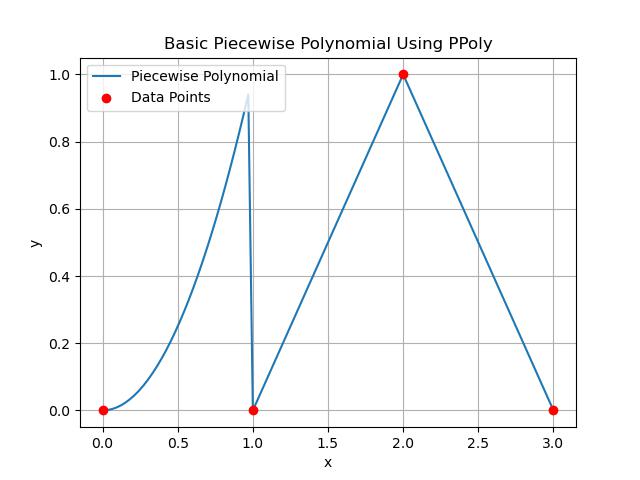
Following is the example of scipy.interpolate.PPoly() function to represent the piecewise polynomial. In this example we define a simple piecewise polynomial and evaluate it at several points −

import numpy as np
import matplotlib.pyplot as plt
from scipy.interpolate import PPoly

# Define breakpoints and polynomial coefficients
x = np.array([0, 1, 2, 3])  # Breakpoints for the intervals
c = np.array([
    [1, 0, 0],  # Coefficients for the first interval [0, 1]: p(x) = 1
    [0, 1, -1], # Coefficients for the second interval [1, 2]: p(x) = x - 1
    [0, 0, 1]   # Coefficients for the third interval [2, 3]: p(x) = (x - 2)^2
])

# Create the piecewise polynomial
pp = PPoly(c, x)

# Evaluate the polynomial at new points
x_new = np.linspace(0, 3, 100)
y_new = pp(x_new)

# Plot the piecewise polynomial
plt.plot(x_new, y_new, label='Piecewise Polynomial')
plt.scatter(x, pp(x), color='red', label='Data Points', zorder=5)
plt.xlabel('x')
plt.ylabel('y')
plt.legend()
plt.title('Basic Piecewise Polynomial Using PPoly')
plt.grid()
plt.show()

Here is the output of the scipy.interpolate.PPoly() function basic example −

Differentiating a Piecewise Polynomial

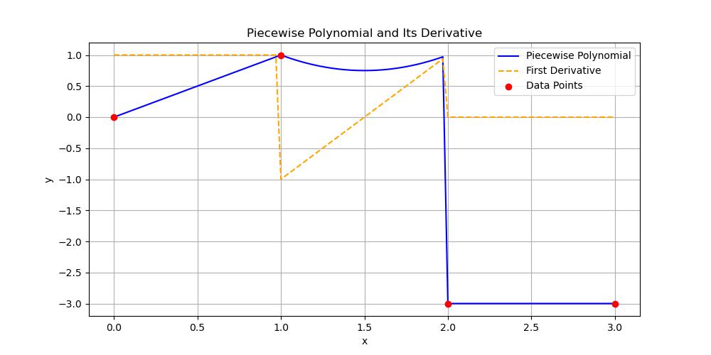
Differentiating a piecewise polynomial involves finding the derivative of each polynomial segment within its defined interval. The resulting piecewise function will describe the rate of change for the overall piecewise polynomial. Following is the example of it −

import numpy as np
import matplotlib.pyplot as plt
from scipy.interpolate import PPoly

# Define breakpoints and polynomial coefficients
x = np.array([0, 1, 2, 3])  # Breakpoints
c = np.array([
    [0, 1, 0],  # Coefficients for the first interval [0, 1]: p(x) = x
    [1, -1, 0], # Coefficients for the second interval [1, 2]: p(x) = -x + 2
    [0, 1, -3]  # Coefficients for the third interval [2, 3]: p(x) = x - 3
])

# Create the piecewise polynomial
pp = PPoly(c, x)

# Evaluate the polynomial and its derivative
x_new = np.linspace(0, 3, 100)
y_new = pp(x_new)
pp_derivative = pp.derivative()  # First derivative
y_derivative = pp_derivative(x_new)

# Plot
plt.figure(figsize=(10, 5))
plt.plot(x_new, y_new, label='Piecewise Polynomial', color='blue')
plt.plot(x_new, y_derivative, label='First Derivative', linestyle='--', color='orange')
plt.scatter(x, pp(x), color='red', label='Data Points', zorder=5)
plt.xlabel('x')
plt.ylabel('y')
plt.legend()
plt.title('Piecewise Polynomial and Its Derivative')
plt.grid()
plt.show()

Here is the output of the scipy.interpolate.PPoly() function which performed Differentialting −

Integrating a Piecewise Polynomial

In this example we compute the integral of a piecewise polynomial over a specific interval −

import numpy as np
import matplotlib.pyplot as plt
from scipy.interpolate import PPoly

# Define breakpoints and polynomial coefficients
x = np.array([0, 1, 2, 3])  # Breakpoints
c = np.array([
    [0, 1, 0],  # Coefficients for the first interval [0, 1]: p(x) = x
    [1, -1, 0], # Coefficients for the second interval [1, 2]: p(x) = -x + 2
    [0, 1, -3]  # Coefficients for the third interval [2, 3]: p(x) = x - 3
])

# Create the piecewise polynomial
pp = PPoly(c, x)

# Evaluate the polynomial and its derivative
x_new = np.linspace(0, 3, 100)
y_new = pp(x_new)
pp_derivative = pp.derivative()  # First derivative
y_derivative = pp_derivative(x_new)

# Plot
plt.figure(figsize=(10, 5))
plt.plot(x_new, y_new, label='Piecewise Polynomial', color='blue')
plt.plot(x_new, y_derivative, label='First Derivative', linestyle='--', color='orange')
plt.scatter(x, pp(x), color='red', label='Data Points', zorder=5)
plt.xlabel('x')
plt.ylabel('y')
plt.legend()
plt.title('Piecewise Polynomial and Its Derivative')
plt.grid()
plt.show()

Here is the output of the scipy.interpolate.PPoly() function which performed Integration −

Integral of piecewise polynomial from 1 to 2: 0.8333333333333333
Integral of piecewise polynomial from 0 to 3: -1.6666666666666667