SciPy - interpolate.NearestNDInterpolator() Function

scipy.interpolate.NearestNDInterpolator() is a function in SciPy which is used for performing nearest-neighbor interpolation on scattered data in N-dimensional space. It assigns values to interpolation points by selecting the value of the nearest data point making it suitable for situations where a blocky or stepwise interpolation is acceptable.

This functiom is straightforward and computationally efficient as it does not compute a smooth surface between points. This approach works well with irregularly spaced data or categorical data where other interpolation methods might not be suitable. Its particularly useful for filling values quickly without complex computation.

Syntax

Following is the syntax of the function scipy.interpolate.NearestNDInterpolator() used for performing nearest-neighbor interpolation −

scipy.interpolate.NearestNDInterpolator(points, values, rescale=False)

Parameters

Below are the parameters of the scipy.interpolate.NearestNDInterpolator() function −

• points(array-like, shape (n, D)): Coordinates of the known data points (e.g., [x, y, z, ...]).
• values(array-like, shape(n,)): Values associated with each point in points.
• rescale(bool, optional): If True then rescales the points to the unit cube before interpolating. This can be helpful if our data has very different scales across dimensions.
• fill_value(float, optional): The value to use for points outside the convex hull of the input points. The default value is np.nan which means that points outside will return NaN.

Return Value

The scipy.interpolate.NearestNDInterpolator() an instance of NearestNDInterpolator which can be called with new coordinates to get interpolated values.

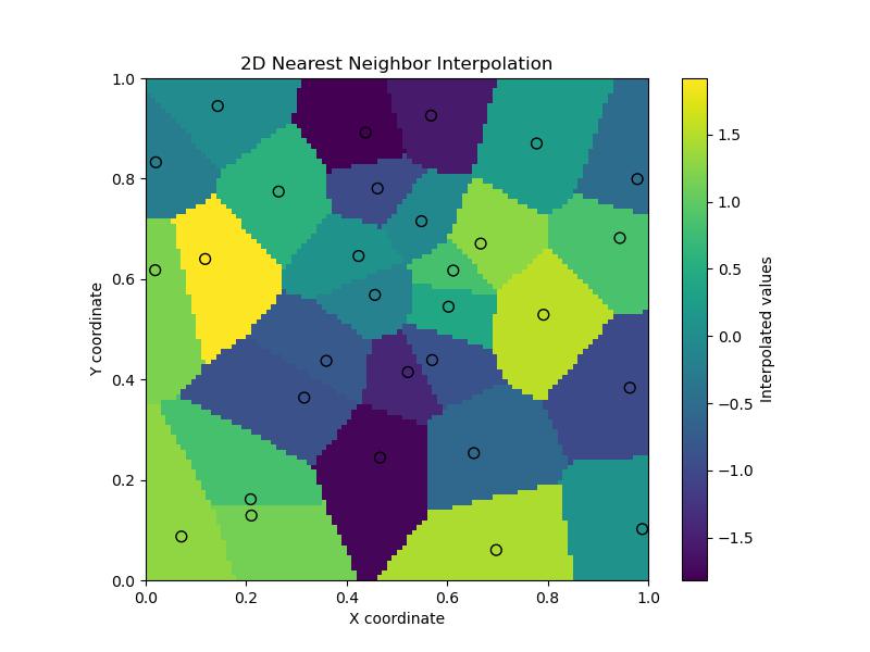
Basic 2D Nearest-Neighbor Interpolation

Following is the example of scipy.interpolate.NearestNDInterpolator() function. This example shows how to use NearestNDInterpolator to interpolate scattered points on a 2D grid −

import numpy as np
import matplotlib.pyplot as plt
from scipy.interpolate import NearestNDInterpolator

# Define some scattered 2D points and their values
np.random.seed(0)  # For reproducibility
points = np.random.rand(30, 2)  # 30 random points in 2D
values = np.sin(points[:, 0] * 10) + np.cos(points[:, 1] * 10)

# Create the NearestNDInterpolator object
interpolator = NearestNDInterpolator(points, values)

# Define a 2D grid for interpolation
grid_x, grid_y = np.mgrid[0:1:100j, 0:1:100j]  # 100x100 grid

# Interpolate on the grid
grid_values = interpolator(grid_x, grid_y)

# Plot the results
plt.figure(figsize=(8, 6))
plt.imshow(grid_values.T, extent=(0, 1, 0, 1), origin='lower', cmap='viridis')
plt.colorbar(label="Interpolated values")
plt.scatter(points[:, 0], points[:, 1], c=values, edgecolor='k', s=50, cmap="viridis")
plt.title("2D Nearest Neighbor Interpolation")
plt.xlabel("X coordinate")
plt.ylabel("Y coordinate")
plt.show()

Here is the output of the scipy.interpolate.NearestNDInterpolator() function basic example −

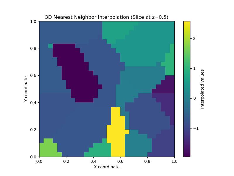
3D Nearest-Neighbor Interpolation

In SciPy we can use scipy.interpolate.NearestNDInterpolator() for nearest-neighbor interpolation in 3D or higher dimensions. This interpolation method assigns each query point the value of the nearest data point by making it especially useful when we want discrete piecewise-constant interpolation without smoothing between values. Below is the example which shows nearest-neighbor interpolation in 3D space using NearestNDInterpolator −

import numpy as np
from scipy.interpolate import NearestNDInterpolator
import matplotlib.pyplot as plt
from mpl_toolkits.mplot3d import Axes3D

# Generate scattered 3D points and their values
np.random.seed(1)
points = np.random.rand(50, 3)  # 50 random points in 3D space
values = np.sin(points[:, 0] * 10) + np.cos(points[:, 1] * 10) + np.sin(points[:, 2] * 10)

# Create the NearestNDInterpolator object
interpolator = NearestNDInterpolator(points, values)

# Define a grid for interpolation
grid_x, grid_y, grid_z = np.mgrid[0:1:30j, 0:1:30j, 0:1:30j]  # 30x30x30 grid

# Interpolate on the grid
grid_values = interpolator(grid_x, grid_y, grid_z)

# Visualize a slice of the 3D grid (for example, at z=0.5)
slice_z = 15  # middle slice for z in a 30x30x30 grid
plt.figure(figsize=(8, 6))
plt.imshow(grid_values[:, :, slice_z], extent=(0, 1, 0, 1), origin='lower', cmap='viridis')
plt.colorbar(label="Interpolated values")
plt.title("3D Nearest Neighbor Interpolation (Slice at z=0.5)")
plt.xlabel("X coordinate")
plt.ylabel("Y coordinate")
plt.show()

Here is the output of the scipy.interpolate.NearestNDInterpolator() function used for 3d interpolation −

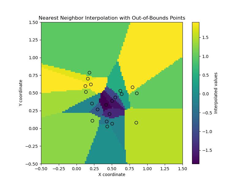
Handling Out-of-Bounds Points

This example uses NearestNDInterpolator to interpolate points on a 2D grid that includes areas outside the convex hull of the original points. The points outside the convex hull will be assigned the value of the nearest point in the data −

import numpy as np
import matplotlib.pyplot as plt
from scipy.interpolate import NearestNDInterpolator

# Generate some scattered points and their values
np.random.seed(2)
points = np.random.rand(20, 2)  # 20 random points in 2D
values = np.sin(points[:, 0] * 10) + np.cos(points[:, 1] * 10)

# Create the NearestNDInterpolator object
interpolator = NearestNDInterpolator(points, values)

# Define a grid that extends beyond the range of `points`
grid_x, grid_y = np.mgrid[-0.5:1.5:100j, -0.5:1.5:100j]  # Extended grid

# Interpolate on the grid
grid_values = interpolator(grid_x, grid_y)

# Plot the results
plt.figure(figsize=(8, 6))
plt.imshow(grid_values.T, extent=(-0.5, 1.5, -0.5, 1.5), origin='lower', cmap="viridis")
plt.colorbar(label="Interpolated values")
plt.scatter(points[:, 0], points[:, 1], c=values, edgecolor='k', s=50, cmap="viridis")
plt.title("Nearest Neighbor Interpolation with Out-of-Bounds Points")
plt.xlabel("X coordinate")
plt.ylabel("Y coordinate")
plt.show()

Here is the output of the scipy.interpolate.NearestNDInterpolator() function which performed outbounds −