SciPy - interpolate.LinearNDInterpolator() Function

scipy.interpolate.LinearNDInterpolator() is a function in SciPy which is used for interpolating scattered data in N-dimensional space. It constructs a piecewise linear interpolation from given data points and their corresponding values.

This LinearNdInterpolator can handle any number of dimensions and is particularly useful for irregularly spaced data. When instantiated with a set of points and values it allows querying at new coordinates by providing interpolated values based on the surrounding data points. This method efficiently finds the simplex containing the query point and computes the interpolated result through linear combinations of the surrounding points.

Syntax

Following is the syntax of the function scipy.interpolate.LinearNDInterpolator() used for interpolating scattered data in N-dimensional space −

scipy.interpolate.LinearNDInterpolator(points, values, xi, method='linear', fill_value=np.nan, rescale=False)

Parameters

Below are the parameters of the scipy.interpolate.LinearNDInterpolator() function −

• points(array-like, shape (n, D)): The coordinates of the data points. Here n is the number of points and D is the dimensionality of the space.
• values(array-like, shape(n,)): The values at each point in points. Each value corresponds to the point defined in points.
• method(str, optional): The interpolation method to use. The default value is 'linear'. For LinearNDInterpolator this parameter is effectively ignored since it only supports linear interpolation.
• fill_value(float, optional): The value to use for points outside the convex hull of the input points. The default value is np.nan which means that points outside will return NaN.

Return Value

The scipy.interpolate.LinearNDInterpolator() function returns an instance of LinearNDInterpolator which can be called as a function to compute interpolated values at specified points.

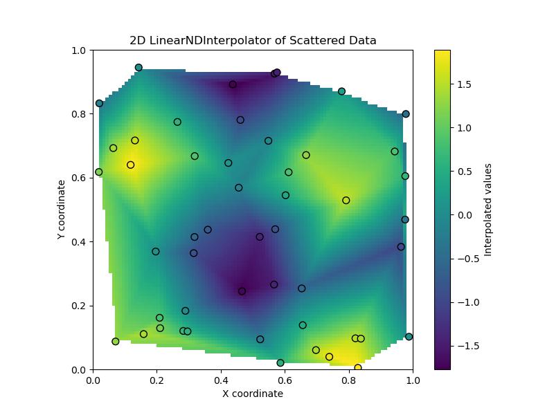
Basic Usage of LinearNDInterpolator in 2D

Following is the example of scipy.interpolate.LinearNDInterpolator() function. In this example we are interpolating data in the with the scattered points −

import numpy as np
import matplotlib.pyplot as plt
from scipy.interpolate import LinearNDInterpolator

# Define some scattered points and their corresponding values
np.random.seed(0)  # For reproducibility
points = np.random.rand(50, 2)  # 50 random points in 2D space
values = np.sin(points[:, 0] * 10) + np.cos(points[:, 1] * 10)  # Assign values based on a sine-cosine function

# Create the LinearNDInterpolator object
interpolator = LinearNDInterpolator(points, values)

# Define a grid where we want to interpolate
grid_x, grid_y = np.mgrid[0:1:100j, 0:1:100j]  # 100x100 grid covering [0, 1] x [0, 1]

# Interpolate on the grid
grid_z = interpolator(grid_x, grid_y)

# Plot the result
plt.figure(figsize=(8, 6))
plt.imshow(grid_z.T, extent=(0, 1, 0, 1), origin='lower', cmap="viridis")
plt.colorbar(label="Interpolated values")
plt.scatter(points[:, 0], points[:, 1], c=values, edgecolor='k', s=50, cmap="viridis")  # Original points
plt.title("2D LinearNDInterpolator of Scattered Data")
plt.xlabel("X coordinate")
plt.ylabel("Y coordinate")
plt.show()

Here is the output of the scipy.interpolate.LinearNDInterpolator() function basic example −

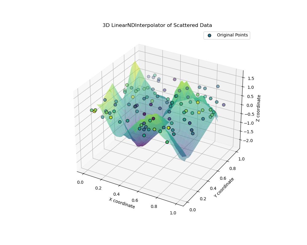
3D Interpolation

Here's an example of performing 3D interpolation using scipy.interpolate.LinearNDInterpolator(). This example shows how to interpolate scattered data points in three dimensions and visualize the result using a 3D surface plot −

import numpy as np
import matplotlib.pyplot as plt
from mpl_toolkits.mplot3d import Axes3D  # For 3D plotting
from scipy.interpolate import LinearNDInterpolator

# Define some scattered 3D points and their corresponding values
np.random.seed(0)  # For reproducibility
num_points = 100
points = np.random.rand(num_points, 3)  # 100 random points in 3D space
values = np.sin(points[:, 0] * 10) + np.cos(points[:, 1] * 10) + np.sin(points[:, 2] * 10)  # Assign values based on a function

# Create the LinearNDInterpolator object
interpolator = LinearNDInterpolator(points, values)

# Define a grid for interpolation
grid_x, grid_y, grid_z = np.mgrid[0:1:30j, 0:1:30j, 0:1:30j]  # 30x30x30 grid covering [0, 1] x [0, 1] x [0, 1]

# Interpolate on the grid
grid_values = interpolator(grid_x, grid_y, grid_z)

# Plot the result
fig = plt.figure(figsize=(10, 8))
ax = fig.add_subplot(111, projection='3d')

# To visualize the interpolation result, we will use scatter for the original points and plot a surface
# For simplicity, we'll plot a scatter of the interpolated values
# You might want to visualize slices of the grid for better understanding in 3D

# Scatter original points
ax.scatter(points[:, 0], points[:, 1], points[:, 2], c=values, edgecolor='k', s=50, label='Original Points')

# Create a surface plot for a slice of the 3D grid (at fixed z = 0.5 for visualization)
slice_z = 0.5
grid_slice = grid_values[:, :, 15]  # Taking a slice at z index 15 (since grid is 30x30x30)

# Create a meshgrid for the slice
X, Y = np.meshgrid(np.linspace(0, 1, 30), np.linspace(0, 1, 30))
ax.plot_surface(X, Y, grid_slice, cmap='viridis', alpha=0.5)

ax.set_title("3D LinearNDInterpolator of Scattered Data")
ax.set_xlabel("X coordinate")
ax.set_ylabel("Y coordinate")
ax.set_zlabel("Z coordinate")
plt.legend()
plt.show()

Here is the output of the scipy.interpolate.LinearNDInterpolator() function used in 3d interpolation −