SciPy - interpolate.krogh_interpolate() Function

scipy.interpolate.krogh_interpolate() is a function that performs polynomial interpolation based on the Krogh or Hermite method. It computes a polynomial that passes exactly through a given set of points and can also interpolate given derivative values at those points. This function is particularly useful when both function values and derivative information for Hermite interpolation are available.

Syntax

Following is the syntax of the function scipy.interpolate.krogh_interpolate() to perform polynomial interpolation −

scipy.interpolate.krogh_interpolate(xi, yi, x, der=0, axis=0)

Parameters

Here are the parameters of the scipy.interpolate.krogh_interpolate() function −

• xi(array-like): 1-D array of known x-values (data points) where interpolation is performed.
• yi(array-like): Array of y-values corresponding to the known x-values. If Hermite interpolation is required then yi can be a 2D array where each row corresponds to the values and their derivatives at the same point.
• x(array-like): Points at which to evaluate the interpolating polynomial i.e., the new x-values where the polynomial is evaluated.
• axis(int, optional): Axis along which to interpolate if yi is multidimensional.
• der(int or list of int, optional): Specifies the order of the derivative to compute. If der=0 then the function returns the interpolated values. If higher-order derivatives are requested then the function returns the corresponding derivatives at the specified points.

Return Value

The scipy.interpolate.krogh_interpolate() function returns the interpolated y-values or the derivatives if der > 0 at the points specified by x.

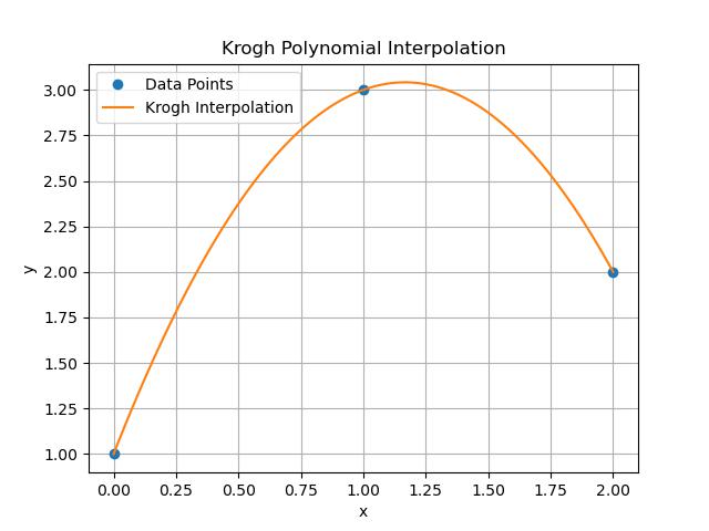
Basic Polynomial Interpolation

Following is the example of using the scipy.interpolate.krogh_interpolate() function which is used to perform polynomial interpolation −

from scipy.interpolate import krogh_interpolate
import numpy as np
import matplotlib.pyplot as plt

# Known data points
xi = np.array([0, 1, 2])
yi = np.array([1, 3, 2])

# Points where we want to evaluate the interpolating polynomial
x_new = np.linspace(0, 2, 100)

# Perform interpolation
y_new = krogh_interpolate(xi, yi, x_new)

# Plot the original points and interpolated values
plt.plot(xi, yi, 'o', label='Data Points')  # Known points
plt.plot(x_new, y_new, label='Krogh Interpolation')  # Interpolated curve
plt.legend()
plt.xlabel('x')
plt.ylabel('y')
plt.title('Krogh Polynomial Interpolation')
plt.grid()
plt.show()

Here is the output of the scipy.interpolate.krogh_interpolate() function −

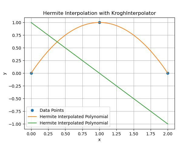
Hermite Interpolation with Derivatives

Hermite interpolation is a type of polynomial interpolation where not only the function values at certain points are provided but also the values of the function's derivatives at those points. Heres an example of how to use KroghInterpolator() function to perform Hermite interpolation when we have derivative information for the points −

import numpy as np
import matplotlib.pyplot as plt
from scipy.interpolate import KroghInterpolator

# Define points (xi) and values/derivatives (yi)
xi = np.array([0, 1, 2])  # x-values of points

# Values and derivatives at each point: [[y0, y0'], [y1, y1'], [y2, y2']]
yi = np.array([[0, 1],  # At x=0, y(0)=0, y'(0)=1
               [1, 0],  # At x=1, y(1)=1, y'(1)=0
               [0, -1]])  # At x=2, y(2)=0, y'(2)=-1

# Create the KroghInterpolator object
interpolator = KroghInterpolator(xi, yi)

# Generate new points for interpolation
x_new = np.linspace(0, 2, 100)

# Interpolate values at the new points
y_new = interpolator(x_new)

# Plot original points and the Hermite interpolated polynomial
plt.plot(xi, yi[:, 0], 'o', label='Data Points')  # Plot data points
plt.plot(x_new, y_new, label='Hermite Interpolated Polynomial')  # Interpolated curve
plt.legend()
plt.xlabel('x')
plt.ylabel('y')
plt.title('Hermite Interpolation with KroghInterpolator')
plt.grid()
plt.show()

Here is the output of the scipy.interpolate.krogh_interpolate() function which is used for Hermite Interpolation −

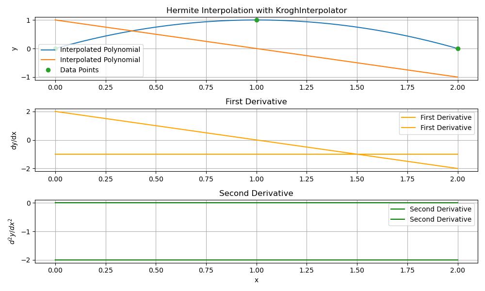
Computing First and Second Derivatives

Here is the example which shows how to compute the first and second derivatives with the help of scipy.interpolate.krogh_interpolate() function −

import numpy as np
import matplotlib.pyplot as plt
from scipy.interpolate import KroghInterpolator

# Define points (xi) and values/derivatives (yi)
xi = np.array([0, 1, 2])  # x-values of points

# Values and derivatives at each point: [[y0, y0'], [y1, y1'], [y2, y2']]
yi = np.array([[0, 1],  # At x=0, y(0)=0, y'(0)=1
               [1, 0],  # At x=1, y(1)=1, y'(1)=0
               [0, -1]])  # At x=2, y(2)=0, y'(2)=-1

# Create the KroghInterpolator object
interpolator = KroghInterpolator(xi, yi)

# Generate new points for interpolation
x_new = np.linspace(0, 2, 100)

# Interpolate values at the new points
y_new = interpolator(x_new)

# Compute first derivative at new points
y_prime = interpolator.derivative(x_new, der=1)

# Compute second derivative at new points
y_double_prime = interpolator.derivative(x_new, der=2)

# Plot original function and its first and second derivatives
plt.figure(figsize=(10, 6))

# Plot the interpolated polynomial
plt.subplot(3, 1, 1)
plt.plot(x_new, y_new, label="Interpolated Polynomial")
plt.plot(xi, yi[:, 0], 'o', label="Data Points")
plt.title('Hermite Interpolation with KroghInterpolator')
plt.ylabel('y')
plt.legend()
plt.grid()

# Plot the first derivative
plt.subplot(3, 1, 2)
plt.plot(x_new, y_prime, label="First Derivative", color='orange')
plt.title('First Derivative')
plt.ylabel("dy/dx")
plt.legend()
plt.grid()

# Plot the second derivative
plt.subplot(3, 1, 3)
plt.plot(x_new, y_double_prime, label="Second Derivative", color='green')
plt.title('Second Derivative')
plt.xlabel('x')
plt.ylabel(r"$d^2y/dx^2$")
plt.legend()
plt.grid()

plt.tight_layout()
plt.show()

Here is the output of the scipy.interpolate.krogh_interpolate() function which is used to compute first and second order derivatives −