SciPy - interpolate.interpn() Function

---

---

scipy.interpolate.interpn() is a multidimensional interpolation function that allows interpolating data on a regular grid in multiple dimensions. When given the grid coordinates and corresponding values then it can interpolate values at arbitrary points within the grids bounds.

It supports various interpolation methods such as 'linear', 'nearest' and 'splinef2d'. Unlike Rbf() function which works for scattered data where as interpn() function is specifically for data on a structured grid.

Its highly useful in fields requiring interpolation on multidimensional grids such as image processing, physics simulations and geographical data analysis where data is defined at regular intervals across multiple axes.

Syntax

Following is the syntax of the function scipy.interpolate.interpn() which is used to do mutli dimensional interpolation −

scipy.interpolate.interpn(points, values, xi, method='linear', bounds_error=True, fill_value=nan)

Parameters

Following are the parameters of the scipy.interpolate.interpn() function −

• points: Sequence of arrays, each array defining the grid points for that dimension. This should match the dimensions of values.
• values: N-dimensional array of values on the grid defined by points.
• xi: Array of points at which to interpolate. Each row represents a point and each column corresponds to a dimension.
• method: Interpolation method; options are 'linear', 'nearest' and 'splinef2d'. Default value is 'linear'.
• bounds_error: If True then raises an error when xi is out of bounds. If False then out-of-bounds points are assigned the fill_value.
• fill_value: Value to use for out-of-bounds points if bounds_error=False. Default value is nan.

Return Value

The scipy.interpolate.interpn() function returns an array of interpolated values at the xi points.

1D Interpolation

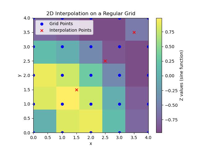
Following is the example of scipy.interpolate.interpn() function in which well interpolate the values on a 2D grid to find values at intermediate points −

import numpy as np
from scipy.interpolate import interpn
import matplotlib.pyplot as plt

# Define a regular 2D grid
x = np.linspace(0, 4, 5)  # x-coordinates of the grid
y = np.linspace(0, 4, 5)  # y-coordinates of the grid
X, Y = np.meshgrid(x, y)

# Define some values on the grid (e.g., using a sine function)
Z = np.sin(np.sqrt(X**2 + Y**2))

# New points where we want to interpolate values
xi = np.array([[1.5, 1.5], [2.5, 2.5], [3.5, 3.5]])

# Perform interpolation
zi = interpn((x, y), Z, xi, method='linear')

# Display results
print("Interpolated values at xi:", zi)

# Plot the grid and interpolation points
plt.imshow(Z, extent=(0, 4, 0, 4), origin='lower', cmap='viridis', alpha=0.7)
plt.colorbar(label="Z values (sine function)")
plt.scatter(X, Y, color='blue', marker='o', label='Grid Points')
plt.scatter(xi[:, 0], xi[:, 1], color='red', marker='x', label='Interpolation Points')
plt.legend()
plt.title("2D Interpolation on a Regular Grid")
plt.xlabel("x")
plt.ylabel("y")
plt.show()

Here is the output of the scipy.interpolate.interpn() function used for simple 2d interpolation −

Interpolated values at xi: [ 0.71733399 -0.3696485  -0.84892675]

3D Interpolation

To perform 3D interpolation on a regular grid using scipy.interpolate.interpn() we have to create a 3D grid of data and then interpolate at specific points within this grid. In this example we will define a 3D grid and calculate function values on it then use interpn() function to find values at desired points in between −

import numpy as np
from scipy.interpolate import interpn
import matplotlib.pyplot as plt
from mpl_toolkits.mplot3d import Axes3D

# Define a regular 3D grid
x = np.linspace(0, 4, 5)  # x-coordinates of the grid
y = np.linspace(0, 4, 5)  # y-coordinates of the grid
z = np.linspace(0, 4, 5)  # z-coordinates of the grid
X, Y, Z = np.meshgrid(x, y, z, indexing="ij")

# Define values on the grid (e.g., based on a radial function)
values = np.sin(np.sqrt(X**2 + Y**2 + Z**2))

# Points where we want to interpolate values
xi = np.array([[1.5, 1.5, 1.5], [2.5, 2.5, 2.5], [3.5, 3.5, 3.5]])

# Perform 3D interpolation
vi = interpn((x, y, z), values, xi, method='linear')

# Display interpolated values
print("Interpolated values at xi:", vi)

# Visualization
fig = plt.figure()
ax = fig.add_subplot(111, projection='3d')

# Plot the original grid points
ax.scatter(X, Y, Z, c=values.ravel(), cmap='viridis', marker='o', label='Grid Points')

# Plot interpolation points
ax.scatter(xi[:, 0], xi[:, 1], xi[:, 2], color='red', marker='x', label='Interpolation Points')

# Labels and legend
ax.set_xlabel('X')
ax.set_ylabel('Y')
ax.set_zlabel('Z')
ax.legend()
plt.title("3D Interpolation on a Regular Grid")
plt.show()

Here is the output of the scipy.interpolate.interpn() function used for 3d interpolation −

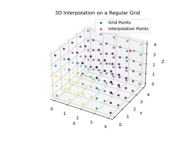
Interpolated values at xi: [ 0.37598905 -0.83693641 -0.15450123]

4D Interpolation

In 4D interpolation we have to interpolate values on a regular grid in four dimensions. For this scipy.interpolate.interpn() function is a good choice when data points are defined on a regularly spaced 4D grid. Here's an example where we define a 4D grid and interpolate values at specific intermediate points −

import numpy as np
from scipy.interpolate import interpn

# Define a 4D regular grid
x = np.linspace(0, 1, 5)  # 5 points along x-axis
y = np.linspace(0, 1, 5)  # 5 points along y-axis
z = np.linspace(0, 1, 5)  # 5 points along z-axis
w = np.linspace(0, 1, 5)  # 5 points along w-axis

# Create a grid of values for each axis
X, Y, Z, W = np.meshgrid(x, y, z, w, indexing='ij')

# Define a function for values on this 4D grid
# Here, let's use a simple function of x, y, z, w
values = np.sin(np.pi * X) * np.cos(np.pi * Y) * np.sin(np.pi * Z) * np.cos(np.pi * W)

# Define new points for interpolation (within the grid bounds)
xi = np.array([
    [0.2, 0.2, 0.2, 0.2],
    [0.5, 0.5, 0.5, 0.5],
    [0.8, 0.8, 0.8, 0.8]
])

# Perform 4D interpolation using 'linear' method
interpolated_values = interpn((x, y, z, w), values, xi, method='linear')

# Display results
print("Interpolation points (xi):", xi)
print("Interpolated values at xi:", interpolated_values)

Following is the output of the scipy.interpolate.interpn() function used for 4d interpolation −

Interpolation points (xi): [[0.2 0.2 0.2 0.2]
 [0.5 0.5 0.5 0.5]
 [0.8 0.8 0.8 0.8]]
Interpolated values at xi: [1.87607734e-01 3.74939946e-33 1.87607734e-01]