SciPy - interpolate.interp1d() Function

The scipy.interpolate.interp1d() is a function which creates a one-dimensional piecewise linear or spline interpolating function based on given data points. It takes input arrays x i.e., data points and y i.e., corresponding values and generates a callable function that estimates the values at any specified points within the range of x.

This function supports various interpolation methods such as linear, nearest, zero, cubic and others. Users can also specify behavior for extrapolation beyond the provided data points. This function is particularly useful for tasks requiring interpolation of sampled data which allows for smooth estimations of values between known data points.

Syntax

Following is the syntax of using the scipy.interpolate.interp1d() function −

interp1d(x, y, kind='linear', axis=-1, copy=True, bounds_error=None, fill_value=nan, assume_sorted=False)[source]

Below are the parameters of the scipy.interpolate.interp1d() function −

• x(array-like): The input data points where the function values are known
• y(array-like): The corresponding values of the function at each point in x.
• kind(str or int, optional): The type of interpolation to use. Options include 'linear', 'nearest', 'zero', 'slinear', 'quadratic', 'cubic', etc.
the parameters of BarycentricInterpolator()
• axis(int, optional): The axis along which to interpolate. This is useful for multi-dimensional arrays. The default value is -1.
• copy(bool, optional): Standard deviation of ydata with the default value True. If provided then this is used as weights in the fitting process. If absolute_sigma is False then it is relative weights; if True then the weights are absolute values.
• bounds_error(bool, optional): If True then raise an error when interpolating outside the bounds of the input data. If False then use fill_value for out-of-bounds input. The default value is None.
• fill_value(float or 'extrapolate', optional): The value to return for points outside the range of x if bounds_error is False. Can also be set to 'extrapolate' to enable extrapolation. It's default value is np.nan.
• assume_sorted(bool,optional): If True then assumes that x is sorted in ascending order which can improve performance and the default value is False.

Return Value

The scipy.interpolate.interp1d() function returns an interpolation function that can be used to compute interpolated values based on the provided data points.

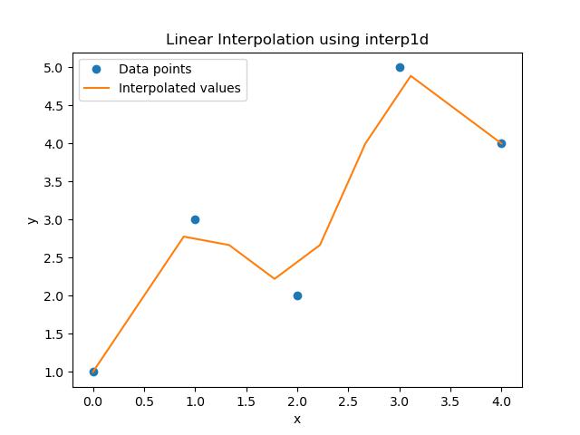
Basic Linear Interpolation

Following is the example which will create a linear interpolation function using scipy.interpolate.interp1d() based on a set of sample data points. We will then use this function to evaluate interpolated values at new x-coordinates −

import numpy as np
from scipy.interpolate import interp1d
import matplotlib.pyplot as plt

# Sample data points
x = np.array([0, 1, 2, 3, 4])
y = np.array([1, 3, 2, 5, 4])

# Create the interpolation function using linear interpolation
f = interp1d(x, y, kind='linear')

# Define new x values for interpolation
x_new = np.linspace(0, 4, num=10)
y_new = f(x_new)  # Evaluate the interpolation function

# Plot the results
plt.plot(x, y, 'o', label='Data points')
plt.plot(x_new, y_new, '-', label='Interpolated values')
plt.legend()
plt.xlabel('x')
plt.ylabel('y')
plt.title('Linear Interpolation using interp1d')
plt.show()

Below is the output of the scipy.interpolate.interp1d() function which is used to perform basic linear interpolation −

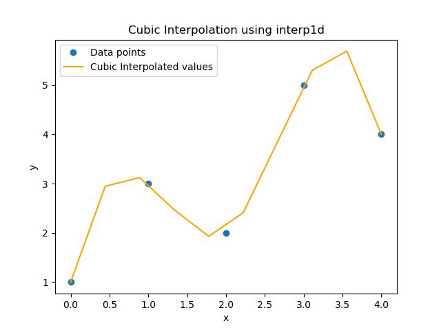
Cubic Interpolation

The Cubic Interpolation is particularly useful when we want to estimate values in a more visually appealing way. In this example we will use cubic interpolation to create a smoother curve through the data points −

import numpy as np
from scipy.interpolate import interp1d
import matplotlib.pyplot as plt

# Sample data points
x = np.array([0, 1, 2, 3, 4])
y = np.array([1, 3, 2, 5, 4])

# Create the interpolation function using cubic interpolation
f_cubic = interp1d(x, y, kind='cubic')

# Define new x values for interpolation
x_new = np.linspace(0, 4, num=10)
y_new = f_cubic(x_new)  # Evaluate the interpolation function
# Define new x values for interpolation
y_cubic = f_cubic(x_new)  # Evaluate the cubic interpolation function

# Plot the results
plt.plot(x, y, 'o', label='Data points')
plt.plot(x_new, y_cubic, '-', label='Cubic Interpolated values', color='orange')
plt.legend()
plt.xlabel('x')
plt.ylabel('y')
plt.title('Cubic Interpolation using interp1d')
plt.show()

Below is the output of the scipy.interpolate.interp1d() function which is used to perform cubic interpolation −

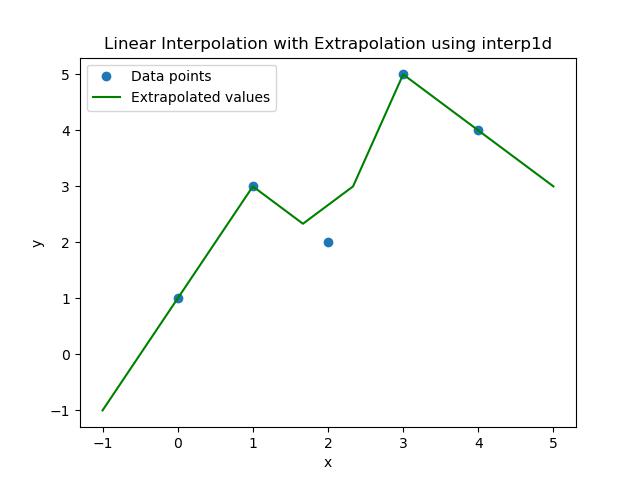
Extrapolation

In this example we will show how to use interp1d() for extrapolation which allows us to predict values outside the range of the provided data points. We will set the fill_value parameter to specify how to handle points outside the input range. −

import numpy as np
from scipy.interpolate import interp1d
import matplotlib.pyplot as plt

# Sample data points
x = np.array([0, 1, 2, 3, 4])
y = np.array([1, 3, 2, 5, 4])

# Create the interpolation function with extrapolation enabled
f_extrapolate = interp1d(x, y, kind='linear', fill_value='extrapolate')

# Define new x values, including values outside the original range
x_new_extrap = np.linspace(-1, 5, num=10)
y_extrapolate = f_extrapolate(x_new_extrap)  # Evaluate the interpolation function

# Plot the results
plt.plot(x, y, 'o', label='Data points')
plt.plot(x_new_extrap, y_extrapolate, '-', label='Extrapolated values', color='green')
plt.legend()
plt.xlabel('x')
plt.ylabel('y')
plt.title('Linear Interpolation with Extrapolation using interp1d')
plt.show()

Following is the output of the scipy.interpolate.interp1d() function which is used to perform Extrapolation −