SciPy - interpolate.griddata() Function

scipy.interpolate.griddata() is a function in SciPy used for interpolating scattered data points onto a structured grid. It takes scattered data with known values at specific points in space and estimates values on a grid of target points. We can provide the function with the coordinates of known points (points), their values (values) and the coordinates of target points (xi).

This function supports three interpolation methods such as linear, nearest and cubic. This function is especially useful in scientific and engineering applications where we need to convert irregularly spaced data into a structured format for analysis or visualization.

Syntax

Following is the syntax of the function scipy.interpolate.griddata() used for interpolating scattered data points −

scipy.interpolate.griddata(points, values, xi, method='linear', fill_value=np.nan, rescale=False)

Parameters

Below are the parameters of the scipy.interpolate.griddata() function −

• points(array-like, shape (n, D)): This is an array of coordinates for the input data points.
• values(array-like, shape(n,)): The values associated with each of the input data points in points. Each entry in values corresponds to the respective entry in points.
• xi(array-like, shape (m, D)): The coordinates where we want to interpolate the data. For example in 2D, this could be a meshgrid created using np.mgrid.
• fill_value(float, optional): This value is used to fill in locations where the interpolation cannot be performed typically for points that fall outside the convex hull of the input points.
• rescale(bool, optional): If set to True then the input points are rescaled to fit within a unit cube before performing the interpolation. This can be useful if the input points have significantly different scales across dimensions.

Return Value

The scipy.interpolate.griddata() function returns an array of interpolated values at the points specified by xi.

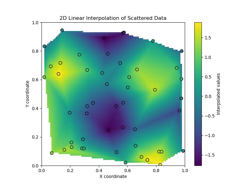
Linear Interpolation on a 2D Grid

Following is the example of scipy.interpolate.griddata() function which is used to perform linear interpolation on a 2D grid. Here we'll take scattered data points, assign values to each and then interpolate these values onto a regular grid. This helps create a smooth approximation of the values over the entire grid −

import numpy as np
from scipy.interpolate import griddata
import matplotlib.pyplot as plt

# Define some random scattered points and corresponding values
np.random.seed(0)  # For reproducibility
points = np.random.rand(50, 2)  # 50 random points in 2D space
values = np.sin(points[:, 0] * 10) + np.cos(points[:, 1] * 10)  # Assign a value to each point

# Define a grid where we want to interpolate
grid_x, grid_y = np.mgrid[0:1:100j, 0:1:100j]  # 100x100 grid covering [0, 1] x [0, 1]

# Perform linear interpolation
grid_z = griddata(points, values, (grid_x, grid_y), method='linear')

# Plot the result
plt.figure(figsize=(8, 6))
plt.imshow(grid_z.T, extent=(0, 1, 0, 1), origin='lower', cmap="viridis")
plt.colorbar(label="Interpolated values")
plt.scatter(points[:, 0], points[:, 1], c=values, edgecolor='k', s=50, cmap="viridis")  # Original points
plt.title("2D Linear Interpolation of Scattered Data")
plt.xlabel("X coordinate")
plt.ylabel("Y coordinate")
plt.show()

Here is the output of the scipy.interpolate.griddata() function basic example −

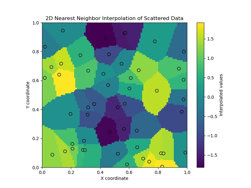
Nearest Neighbor Interpolation on griddata

Here's an example of using nearest neighbor interpolation on a 2D grid with scipy.interpolate.griddata(). This method assigns to each grid point the value of the closest scattered data point which can be useful when we want a blocky or non-smoothed result −

import numpy as np
from scipy.interpolate import griddata
import matplotlib.pyplot as plt

# Define some random scattered points and their corresponding values
np.random.seed(0)  # For reproducibility
points = np.random.rand(50, 2)  # 50 random points in 2D space
values = np.sin(points[:, 0] * 10) + np.cos(points[:, 1] * 10)  # Assign values based on sine-cosine function

# Define a grid where we want to interpolate
grid_x, grid_y = np.mgrid[0:1:100j, 0:1:100j]  # 100x100 grid covering [0, 1] x [0, 1]

# Perform nearest neighbor interpolation
grid_z = griddata(points, values, (grid_x, grid_y), method='nearest')

# Plot the result
plt.figure(figsize=(8, 6))
plt.imshow(grid_z.T, extent=(0, 1, 0, 1), origin='lower', cmap="viridis")
plt.colorbar(label="Interpolated values")
plt.scatter(points[:, 0], points[:, 1], c=values, edgecolor='k', s=50, cmap="viridis")  # Original points
plt.title("2D Nearest Neighbor Interpolation of Scattered Data")
plt.xlabel("X coordinate")
plt.ylabel("Y coordinate")
plt.show()

Here is the output of the scipy.interpolate.griddata() function used to perfrom Nearest Neighbor Interpolation −

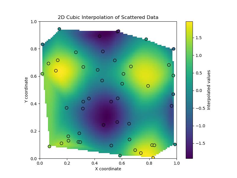
Cubic Interpolation on griddata

Cubic interpolation only works in 2D and it produces smoother results than linear interpolation. Here is the example which geneartes the cubic interpolation on griddata −

import numpy as np
from scipy.interpolate import griddata
import matplotlib.pyplot as plt

# Define some random scattered points and their corresponding values
np.random.seed(0)  # For reproducibility
points = np.random.rand(50, 2)  # 50 random points in 2D space
values = np.sin(points[:, 0] * 10) + np.cos(points[:, 1] * 10)  # Assign values based on sine-cosine function

# Define a grid where we want to interpolate
grid_x, grid_y = np.mgrid[0:1:100j, 0:1:100j]  # 100x100 grid covering [0, 1] x [0, 1]

# Perform cubic interpolation
grid_z = griddata(points, values, (grid_x, grid_y), method='cubic')

# Plot the result
plt.figure(figsize=(8, 6))
plt.imshow(grid_z.T, extent=(0, 1, 0, 1), origin='lower', cmap="viridis")
plt.colorbar(label="Interpolated values")
plt.scatter(points[:, 0], points[:, 1], c=values, edgecolor='k', s=50, cmap="viridis")  # Original points
plt.title("2D Cubic Interpolation of Scattered Data")
plt.xlabel("X coordinate")
plt.ylabel("Y coordinate")
plt.show()

Here is the output of the scipy.interpolate.griddata() function used for cubic interpolation −