SciPy - interpolate.CubicSpline() Function

scipy.interpolate.CubicSpline() is a function in SciPy that performs cubic spline interpolation. This method for constructing smooth curves through a set of points. When the given arrays of x and y coordinates then CubicSpline() creates a piecewise cubic polynomial that passes through each data point with continuous first and second derivatives.

The users can control boundary conditions such as natural i.e., second derivative is zero at endpoints or clamped i.e., specifying first derivatives at endpoints. The result is an interpolated function that can estimate values at intermediate points with high accuracy and smoothness by making it ideal for smooth data approximation.

Syntax

Following is the syntax of the function scipy.interpolate.CubicSpline() to perform cubic spline interpolation −

CubicSpline(x, y, axis=0, bc_type='not-a-knot', extrapolate=None)

Parameters

Below are the parameters of the scipy.interpolate.CubicSpline() function −

• x(array-like, shape(n,)): The x-coordinates of the data points. They must be in strictly increasing order.
• y(array-like, shape(n,)):The y-coordinates of the data points. This can be multidimensional. The interpolation is performed along the specified axis.
• axis(int, optional): This specifies the axis in the y array that corresponds to the x coordinates. This allows for multi-dimensional y arrays where interpolation is only along the specified axis. The default value is 0.
• bc_type(string or 2-tuple, optional): Defines the boundary conditions such as not-a-knot, clamped, natural
• extrapolate(bool or 'periodic', optional): This parameter specifies whether to extrapolate the spline outside of the data range.

Return Value

The scipy.interpolate.CubicSpline() function returns an object that represents a cubic spline interpolation of the input data (x, y).

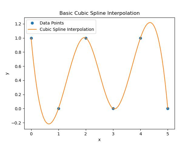
Basic Interpolation

Following is the example of scipy.interpolate.CubicSpline() function for performing the cubic spline interpolation. This example shows how to create a smooth curve that connects each point smoothly which is ideal for data fitting and analysis −

import numpy as np
import matplotlib.pyplot as plt
from scipy.interpolate import CubicSpline

# Sample data points
x = np.array([0, 1, 2, 3, 4, 5])
y = np.array([1, 0, 1, 0, 1, 0])

# Create cubic spline interpolation
cs = CubicSpline(x, y)

# Generate new x values for a smooth curve
x_new = np.linspace(0, 5, 100)
y_new = cs(x_new)

# Plot the original data points and the cubic spline
plt.plot(x, y, 'o', label='Data Points')
plt.plot(x_new, y_new, label='Cubic Spline Interpolation')
plt.xlabel('x')
plt.ylabel('y')
plt.legend()
plt.title('Basic Cubic Spline Interpolation')
plt.show()

Here is the output of the scipy.interpolate.CubicSpline() function basic example −

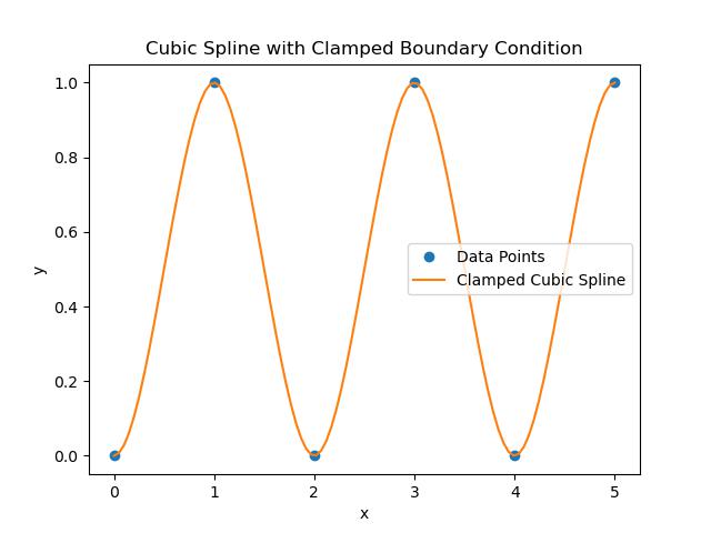
Clamped Boundary Condition

In a clamped boundary condition the spline's first derivative i.e., slope is specified at both endpoints. This can be useful when we know the slope at the start and end points of the data. Heres how to apply the clamped condition in a CubicSpline interpolation −

import numpy as np
import matplotlib.pyplot as plt
from scipy.interpolate import CubicSpline

# Sample data points
x = np.array([0, 1, 2, 3, 4, 5])
y = np.array([0, 1, 0, 1, 0, 1])

# Specify the slopes (first derivatives) at the endpoints
# Here, let's assume we want a slope of 0 at both ends
bc_type = ((1, 0.0), (1, 0.0))  # (1, slope) specifies the derivative order and value

# Create cubic spline with clamped boundary condition
cs = CubicSpline(x, y, bc_type=bc_type)

# Generate new x values for smooth curve
x_new = np.linspace(0, 5, 100)
y_new = cs(x_new)

# Plot the original data points and the cubic spline with clamped condition
plt.plot(x, y, 'o', label='Data Points')
plt.plot(x_new, y_new, label='Clamped Cubic Spline')
plt.xlabel('x')
plt.ylabel('y')
plt.legend()
plt.title('Cubic Spline with Clamped Boundary Condition')
plt.show()

Here is the output of the scipy.interpolate.CubicSpline() function performed clamped boundary −

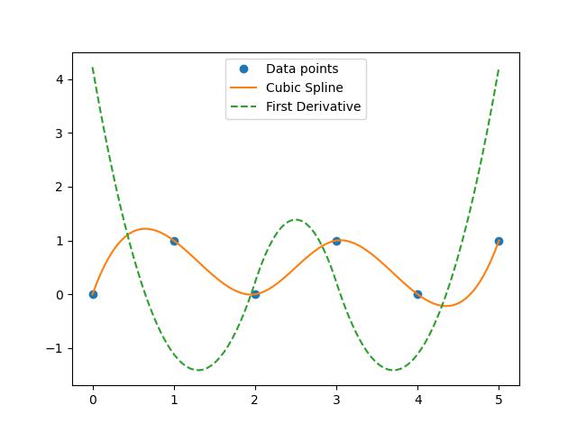
Calculating the Derivative

In this example we calculate and visualize the first derivative of the cubic spline −

import numpy as np
import matplotlib.pyplot as plt
from scipy.interpolate import CubicSpline

# Sample data points
x = np.array([0, 1, 2, 3, 4, 5])
y = np.array([0, 1, 0, 1, 0, 1])

# Specify the slopes (first derivatives) at the endpoints
# Here, let's assume we want a slope of 0 at both ends
bc_type = ((1, 0.0), (1, 0.0))  # (1, slope) specifies the derivative order and value

# Create cubic spline with clamped boundary condition
cs = CubicSpline(x, y, bc_type=bc_type)

# Generate new x values for smooth curve
x_new = np.linspace(0, 5, 100)
y_new = cs(x_new)

# Plot the original data points and the cubic spline with clamped condition
plt.plot(x, y, 'o', label='Data Points')
plt.plot(x_new, y_new, label='Clamped Cubic Spline')
plt.xlabel('x')
plt.ylabel('y')
plt.legend()
plt.title('Cubic Spline with Clamped Boundary Condition')
plt.show()

Here is the output of the scipy.interpolate.CubicSpline() function used to performed Derivative−