SciPy - interpolate.CloughTocher2DInterpolator() Function

scipy.interpolate.CloughTocher2DInterpolator() is a function in SciPy used for smooth interpolation on scattered 2D data. Based on the Clough-Tocher scheme it creates a continuously differentiable surface over triangular tessellations of the input points. This function is particularly useful for complex surfaces where standard grid-based interpolation is insufficient.

This function employs piecewise cubic polynomials over Delaunay triangulation by allowing for an accurate fit even on irregularly spaced data. Users can specify options like interpolation tolerance for more control. Its ideal for applications in computational geometry, computer graphics and surface modeling where smooth interpolation is essential.

Syntax

Following is the syntax of the function scipy.interpolate.CloughTocher2DInterpolator() used for smooth interpolation on scattered 2D data −

CloughTocher2DInterpolator(points, values, fill_value=np.nan, tol=1e-06, maxiter=400, rescale=False)

Parameters

Below are the parameters of the scipy.interpolate.CloughTocher2DInterpolator() function −

• points(array-like, shape (n, D)): 2-D array of data point coordinates or a precomputed Delaunay triangulation.
• values(float or complex, shape (npoints, )): An array of shape (n,) containing the values at the corresponding points. Each value corresponds to a point defined in points.
• fill_value(float, optional): This is the value used to fill in the interpolated values for points outside the convex hull of the input points. If the interpolation is requested at a point outside the domain this value will be returned.
• tol(float, optional): Tolerance for determining if a point is close enough to an input point. Smaller values can lead to more accurate results but may increase computational time.
• maxiter(int, optional): Maximum number of iterations allowed for the optimization algorithm used in the interpolation.
• rescale(bool, optional): If True then the input data will be rescaled to improve the conditioning of the interpolation. This can be helpful if the input data spans several orders of magnitude.

Return Value

The scipy.interpolate.CloughTocher2DInterpolator() function returns an interpolation object which allows us to interpolate values at new 2D points based on the input data.

Basic Interpolation on a Grid

Following is the example of scipy.interpolate.CloughTocher2DInterpolator() function. This example shows how to interpolate values within a 2D grid using known points −

from scipy.interpolate import CloughTocher2DInterpolator
import numpy as np

# Define known points (x, y) and their values
points = np.array([[0, 0], [1, 0], [0, 1], [1, 1], [0.5, 0.5]])
values = np.array([0, 1, 1, 0, 0.5])

# Create the interpolator
interpolator = CloughTocher2DInterpolator(points, values)

# Interpolate at a new point within the convex hull
print("Interpolated value at (0.75, 0.25):", interpolator(0.75, 0.25))

# Interpolate at a point outside the convex hull
print("Interpolated value at (1.5, 1.5):", interpolator(1.5, 1.5))  # Returns NaN or fill_value

Here is the output of the scipy.interpolate.CloughTocher2DInterpolator() function basic example −

Interpolated value at (0.75, 0.25): 0.6401650365046423
Interpolated value at (1.5, 1.5): nan

Interpolation with Custom fill_value

When we need to distinguish points that are interpolated from those that are extrapolated by assigning a clear out-of-bounds value. Below is the example which uses the custom fill_value −

from scipy.interpolate import CloughTocher2DInterpolator
import numpy as np

# Define known points and their corresponding values
points = np.array([[0, 0], [1, 0], [0, 1], [1, 1], [0.5, 0.5]])
values = np.array([0, 1, 1, 0, 0.5])

# Create the CloughTocher2DInterpolator with a custom fill_value
interpolator = CloughTocher2DInterpolator(points, values, fill_value=-1)

# Interpolate at points within the convex hull
print("Interpolated value at (0.25, 0.25):", interpolator(0.25, 0.25))  # Inside the convex hull
print("Interpolated value at (0.75, 0.75):", interpolator(0.75, 0.75))  # Inside the convex hull

# Interpolate at a point outside the convex hull
print("Interpolated value at (1.5, 1.5):", interpolator(1.5, 1.5))  # Outside the convex hull, returns -1

Here is the output of the scipy.interpolate.CloughTocher2DInterpolator() function which is used with fill_value −

Interpolated value at (0.25, 0.25): 0.3598350174937729
Interpolated value at (0.75, 0.75): 0.3598349110543353
Interpolated value at (1.5, 1.5): -1.0

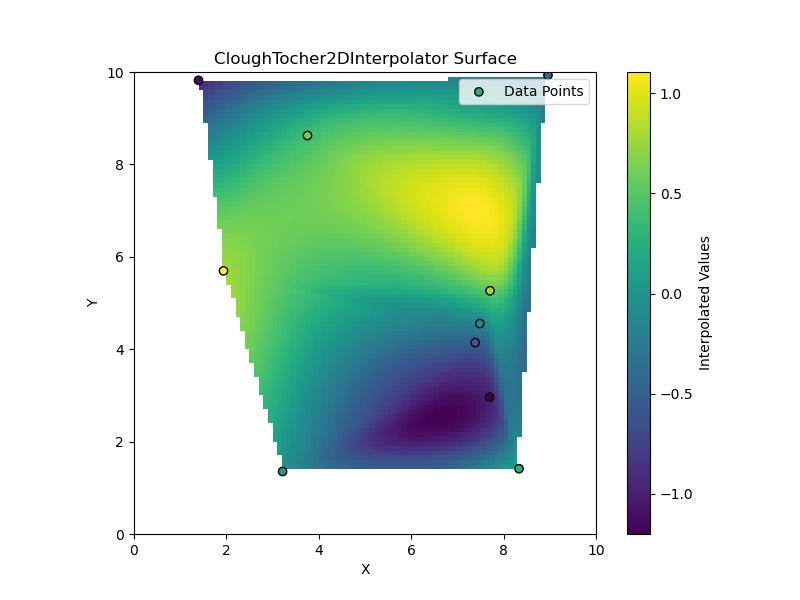
Plotting Interpolated Surface

This example shows how to use CloughTocher2DInterpolator() function to generate an interpolated surface and visualize it −

import numpy as np
import matplotlib.pyplot as plt
from scipy.interpolate import CloughTocher2DInterpolator

# Define irregularly spaced data points
x = np.random.rand(10) * 10
y = np.random.rand(10) * 10
z = np.sin(x) * np.cos(y)

points = np.column_stack((x, y))

# Create the interpolator
interpolator = CloughTocher2DInterpolator(points, z)

# Create a meshgrid for plotting
grid_x, grid_y = np.mgrid[0:10:100j, 0:10:100j]
grid_z = interpolator(grid_x, grid_y)

# Plot the result
plt.figure(figsize=(8, 6))
plt.imshow(grid_z.T, extent=(0, 10, 0, 10), origin='lower', cmap='viridis')
plt.colorbar(label='Interpolated Values')
plt.scatter(x, y, c=z, edgecolor='k', label='Data Points')
plt.legend()
plt.title("CloughTocher2DInterpolator Surface")
plt.xlabel("X")
plt.ylabel("Y")
plt.show()

Here is the output of the scipy.interpolate.CloughTocher2DInterpolator() function which is used with fill_value −