SciPy - interpolate.BPoly() Function

scipy.interpolate.BPoly() is a function in SciPy used to create and evaluate piecewise polynomial functions known as Bernstein polynomials. It allows users to define a polynomial piecewise function based on given coefficients and knots.

This function is particularly useful for interpolation and curve fitting by providing a smooth and continuous representation of data. The BPoly function supports various operations such as evaluating the polynomial at specific points by calculating derivatives and integrating over specified intervals. It is especially valuable in applications requiring high degrees of flexibility and control over polynomial behavior by maintaining numerical stability across intervals.

Syntax

Following is the syntax of the function scipy.interpolate.BPoly() to represent piecewise polynomials −

BPoly(c, x, extrapolate=None, axis=0)

Parameters

Below are the parameters of the scipy.interpolate.BPoly() function −

• c(array-like, shape(k,m)): The coefficients of the polynomial pieces. Each row corresponds to a polynomial, and each column corresponds to a coefficient for decreasing powers of x.
• x(array-like, shape(k,)):The breakpoints or knots where the polynomial pieces are defined. The array must be strictly increasing.
• axis(int, optional): The axis along which the polynomial pieces are defined. This is useful when dealing with multidimensional data.
• extrapolate(bool, optional): Determines whether to allow extrapolation outside the breakpoints. If True, the polynomial will be extended linearly beyond the specified knots. If False, it will return NaN for values outside the range. If None, the default behavior is used based on the value of x.

Return Value

The scipy.interpolate.BPoly() function returns an instance of the BPoly class which represents the piecewise polynomial defined by the coefficients and the breakpoints.

Piecewise Polynomial with BPoly

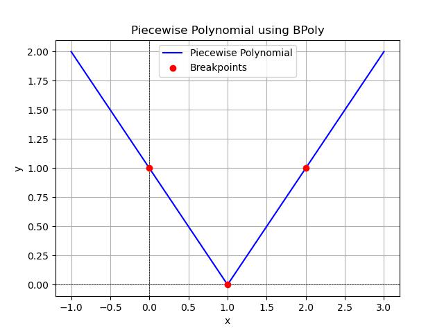
Following is the example of scipy.interpolate.BPoly() function which is used to create and evaluate the piecewise polynomial. In this example we define a simple piecewise polynomial and evaluate it at several points. In this example we will define a piecewise polynomial with two segments, evaluate it over a range of x-values (including points outside the breakpoints) and visualize the result −

import numpy as np
import matplotlib.pyplot as plt
from scipy.interpolate import BPoly

# Define breakpoints (knots)
x = np.array([0, 1, 2])  # Breakpoints

# Define coefficients for the polynomial pieces
# Each row corresponds to a polynomial, ordered by decreasing power of x
c = np.array([[1, 0],    # Polynomial for segment 1: P1(x) = 1 (constant)
              [0, 1]])  # Polynomial for segment 2: P2(x) = x - 1 (linear)

# Create the piecewise polynomial
bp = BPoly(c, x, extrapolate=True)  # Allow extrapolation

# Generate new x values for evaluation, including points outside the breakpoints
x_new = np.linspace(-1, 3, 100)  # Range includes -1 to 3
y_new = bp(x_new)  # Evaluate the piecewise polynomial

# Plot the piecewise polynomial
plt.plot(x_new, y_new, label='Piecewise Polynomial', color='blue')
plt.scatter(x, [1, 0, 1], color='red', label='Breakpoints', zorder=5)
plt.xlabel('x')
plt.ylabel('y')
plt.title('Piecewise Polynomial using BPoly')
plt.legend()
plt.grid()
plt.axhline(0, color='black', lw=0.5, ls='--')  # Horizontal line at y=0
plt.axvline(0, color='black', lw=0.5, ls='--')  # Vertical line at x=0
plt.show()

Here is the output of the scipy.interpolate.BPoly() function basic example −

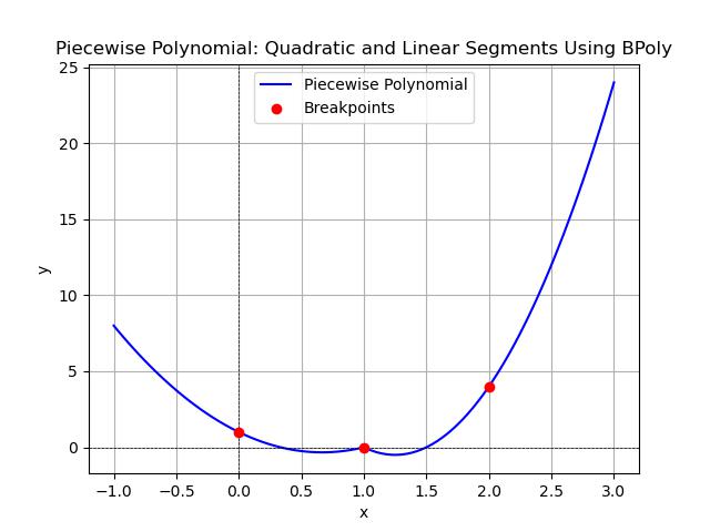
Quadratic and Linear Segments

Quadratic and linear segments can be combined to create a piecewise polynomial function. Each segment can have different properties by allowing for flexibility in modeling various shapes or behaviors. Here's how we can define and evaluate a piecewise polynomial consisting of both quadratic and linear segments −

import numpy as np
import matplotlib.pyplot as plt
from scipy.interpolate import BPoly

# Define breakpoints
breakpoints = np.array([0, 1, 2])  # Breakpoints for the polynomial pieces

# Define coefficients for the polynomial pieces
# Ensure each coefficient set corresponds to one segment and has consistent lengths
coefficients = np.array([[1, -1, 0],  # Coefficients for quadratic segment (1*x^2 - 1*x + 0)
                         [0, -2, 4]])  # Coefficients for linear segment adjusted to fit a quadratic format

# Create the piecewise polynomial
bp = BPoly(c=coefficients.T, x=breakpoints)

# Generate new x values for evaluation
x_new = np.linspace(-1, 3, 100)  # Range includes points outside the breakpoints
y_new = bp(x_new)

# Plot the piecewise polynomial
plt.plot(x_new, y_new, label='Piecewise Polynomial', color='blue')

# Calculate and display breakpoints values for plotting
breakpoint_values = [bp(val) for val in breakpoints]
plt.scatter(breakpoints, breakpoint_values, color='red', label='Breakpoints', zorder=5)  # Show breakpoints

plt.xlabel('x')
plt.ylabel('y')
plt.title('Piecewise Polynomial: Quadratic and Linear Segments Using BPoly')
plt.legend()
plt.grid()
plt.axhline(0, color='black', lw=0.5, ls='--')  # Horizontal line at y=0
plt.axvline(0, color='black', lw=0.5, ls='--')  # Vertical line at x=0
plt.show()

Here is the output of the scipy.interpolate.BPoly() function basic example −