SciPy - interpolate.barycentric_interpolate() Function

scipy.interpolate.barycentric_interpolate() is a function in SciPy which is used to perform polynomial interpolation using the Barycentric Lagrange method. It constructs an interpolating polynomial that passes through a set of given points (xi, yi).

This method is numerically stable and efficient for high-degree polynomials by avoiding common issues like Runge's phenomenon. This function evaluates the interpolated polynomial at specified points.

Syntax

Following is the syntax of the function scipy.interpolate.barycentric_interpolate() to perform polynomial interpolation −

scipy.interpolate.barycentric_interpolate(xi, yi, x, axis=0, *, der=0)

Parameters

Here are the parameters of the scipy.interpolate.barycentric_interpolate() function −

• xi(array-like): 1-D array of data points where interpolation is performed i.e., the x-coordinates of the known data points.
• yi(array-like): 1-D array of values corresponding to the data points i.e., the y-coordinates of the known data points.
• x(array-like): Points at which to evaluate the interpolated values i.e., the x-coordinates where we want the output.
• axis(int, optional): The axis along which to interpolate. For 1-D input this parameter is typically set to 0.
• der(int, optional): If der is set to default value 0 then the function returns the interpolated values. If der is 1 then it returns the first derivative and so on.

Return Value

The scipy.interpolate.barycentric_interpolate() function returns the interpolated values at the specified points x. If der is greater than 0 then it returns the derivatives of the interpolating polynomial at those points.

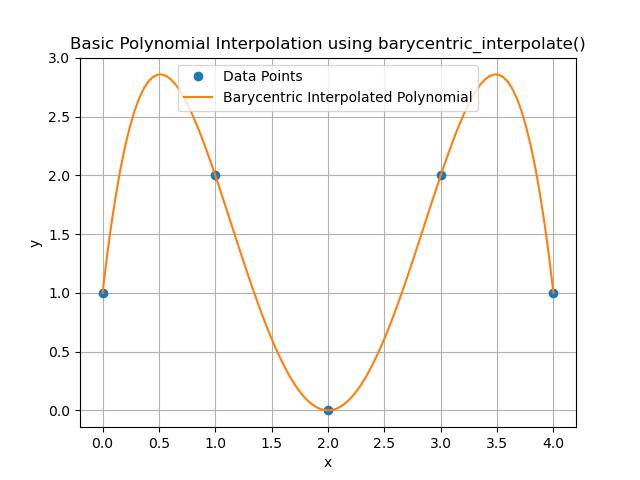
Basic Polynomial Interpolation

Following is the example of using the scipy.interpolate.barycentric_interpolate() function which is used to perform polynomial interpolation −

import numpy as np
import matplotlib.pyplot as plt
from scipy.interpolate import barycentric_interpolate

# Define data points
xi = np.array([0, 1, 2, 3, 4])  # x-values
yi = np.array([1, 2, 0, 2, 1])  # y-values

# Create new x points for interpolation
x_new = np.linspace(0, 4, 100)  # 100 points between 0 and 4

# Perform barycentric interpolation
y_new = barycentric_interpolate(xi, yi, x_new)

# Plot original data points and the interpolated polynomial
plt.plot(xi, yi, 'o', label='Data Points')  # Original points
plt.plot(x_new, y_new, label='Barycentric Interpolated Polynomial')  # Interpolated curve
plt.legend()
plt.xlabel('x')
plt.ylabel('y')
plt.title('Basic Polynomial Interpolation using barycentric_interpolate()')
plt.grid()
plt.show()

Here is the output of the scipy.interpolate.barycentric_interpolate() function −

Evaluating Derivatives

This example effectively shows how to evaluate the derivatives of a polynomial that has been interpolated using the Barycentric method. The derivative plot shows the rate of change of the polynomial across the range defined by the data points −

import numpy as np
from scipy.interpolate import barycentric_interpolate
import matplotlib.pyplot as plt

# Define data points
xi = np.array([0, 1, 2, 3, 4])
yi = np.array([1, 2, 0, 2, 1])

# Points to evaluate the interpolation
x_new = np.linspace(0, 4, 100)  # 100 points between 0 and 4

# Perform interpolation
y_new = barycentric_interpolate(xi, yi, x_new)

# Calculate first derivative
y_deriv = barycentric_interpolate(xi, yi, x_new, der=1)

# Plot original points, the interpolated polynomial, and its derivative
plt.plot(xi, yi, 'o', label='Data Points')  # Original points
plt.plot(x_new, y_new, label='Barycentric Interpolation')  # Interpolated curve
plt.plot(x_new, y_deriv, label='First Derivative', linestyle='--')  # Derivative curve
plt.legend()
plt.xlabel('x')
plt.ylabel('y')
plt.title('Barycentric Interpolation and Its Derivative')
plt.grid()
plt.show()

Here is the output of the scipy.interpolate.barycentric_interpolate() function which is used to evaluate the Derivatives −

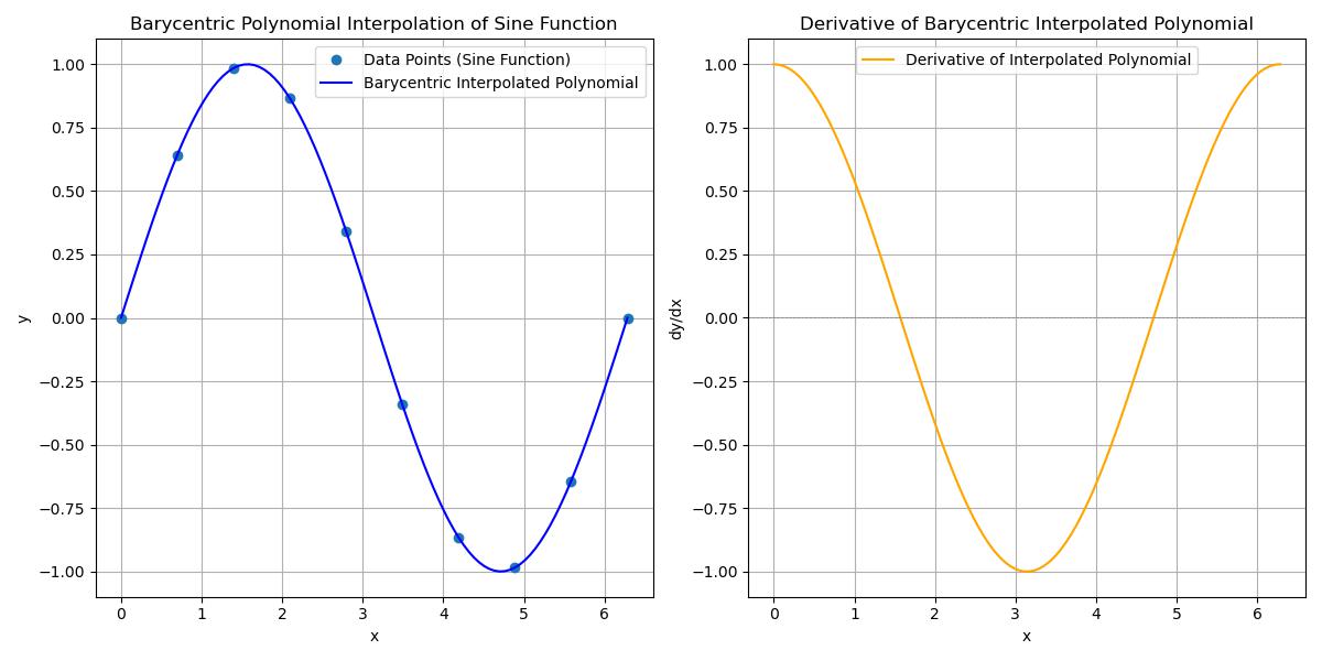
Using More Complex Data Points

Here is an example of the scipy.interpolate.barycentric_interpolate() function which uses the more complex data points −

import numpy as np
import matplotlib.pyplot as plt
from scipy.interpolate import barycentric_interpolate

# Define complex data points based on a sine function
xi = np.linspace(0, 2 * np.pi, 10)  # 10 x-values from 0 to 2p
yi = np.sin(xi)  # Corresponding y-values using the sine function

# Create new x points for interpolation
x_new = np.linspace(0, 2 * np.pi, 100)  # 100 points between 0 and 2p

# Perform barycentric interpolation
y_new = barycentric_interpolate(xi, yi, x_new)

# Define a function to compute the derivative using finite differences
def derivative(xi, yi, x, h=1e-5):
    return (barycentric_interpolate(xi, yi, x + h) - barycentric_interpolate(xi, yi, x - h)) / (2 * h)

# Compute the derivatives at the new x points
y_derivative = derivative(xi, yi, x_new)

# Plot original data points, interpolated polynomial, and its derivative
plt.figure(figsize=(12, 6))

# Subplot for the interpolated polynomial
plt.subplot(1, 2, 1)
plt.plot(xi, yi, 'o', label='Data Points (Sine Function)')  # Original points
plt.plot(x_new, y_new, label='Barycentric Interpolated Polynomial', color='blue')  # Interpolated curve
plt.legend()
plt.xlabel('x')
plt.ylabel('y')
plt.title('Barycentric Polynomial Interpolation of Sine Function')
plt.grid()

# Subplot for the derivative
plt.subplot(1, 2, 2)
plt.plot(x_new, y_derivative, label='Derivative of Interpolated Polynomial', color='orange')
plt.axhline(0, color='grey', lw=0.5, ls='--')  # Horizontal line at y=0
plt.legend()
plt.xlabel('x')
plt.ylabel('dy/dx')
plt.title('Derivative of Barycentric Interpolated Polynomial')
plt.grid()

plt.tight_layout()
plt.show()

Here is the output of the scipy.interpolate.barycentric_interpolate() function using the complex data points −