SciPy - interpolate.Akima1DInterpolator() Function

scipy.interpolate.Akima1DInterpolator() is a function in Python's SciPy library for one-dimensional interpolation using Akima's piecewise cubic interpolation technique. It constructs a series of cubic polynomials that connect the data points while preserving the overall shape and characteristics of the original data.

This function is particularly effective for datasets with abrupt changes as it avoids overshooting and oscillations that can occur with traditional spline methods. The interpolator ensures that the resulting curve is smooth at the data points while being responsive to the local changes in the data by making it suitable for various applications in data analysis and visualization.

Syntax

Following is the syntax of the function scipy.interpolate.Akima1DInterpolator() to perform Akima's piecewise cubic interpolation −

Akima1DInterpolator(x, y, axis=0, extrapolate=None)

Parameters

Below are the parameters of the scipy.interpolate.Akima1DInterpolator() function −

• x: A 1D array-like input representing the x-coordinates of the data points. It must be sorted in increasing order.
• y: A 1D array-like input representing the corresponding y-coordinates. The length of y must match the length of x.
• axis(optional): An integer specifying the axis of the input data along which to interpolate. The default value is 0 which applies to the first axis.
• method (optional): A string specifying the interpolation method. By default it's set to 'akima' indicating the use of Akima's method. Other methods may be specified if available.
• extrapolate(optional): A boolean or a string that determines whether to allow extrapolation. If set to True then the interpolator will perform extrapolation outside the bounds of the input data. If set to False then it will raise an error for values outside the range of x. A string can specify a specific extrapolation method.

Return Value

The scipy.interpolate.Akima1DInterpolator() function returns an interpolator object that can be used to compute interpolated values at any desired x-coordinates within or outside the range of the input data.

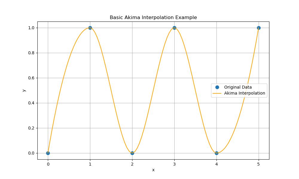
Basic Akima Interpolation

Here's a basic example of using Akima1DInterpolator() for interpolation in Python. This example illustrates how to create an Akima interpolator and visualize the results −

import numpy as np
from scipy.interpolate import Akima1DInterpolator
import matplotlib.pyplot as plt

# Sample data points (x and y)
x = np.array([0, 1, 2, 3, 4, 5])
y = np.array([0, 1, 0, 1, 0, 1])

# Create the Akima interpolator
akima_interpolator = Akima1DInterpolator(x, y)

# Define new x values for interpolation
x_new = np.linspace(0, 5, 100)
y_new = akima_interpolator(x_new)

# Plot the original data points and the interpolated curve
plt.figure(figsize=(10, 6))
plt.plot(x, y, 'o', label='Original Data', markersize=8)
plt.plot(x_new, y_new, label='Akima Interpolation', color='orange')
plt.title('Basic Akima Interpolation Example')
plt.xlabel('x')
plt.ylabel('y')
plt.legend()
plt.grid()
plt.show()

Here is the output of the scipy.interpolate.Akima1DInterpolator() function −

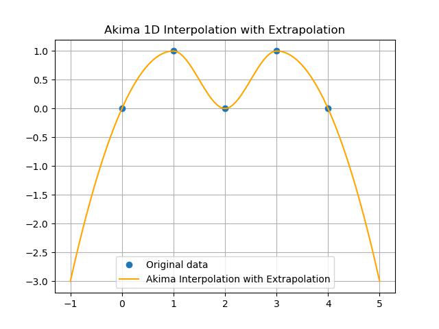
Extrapolation with Akima Interpolation

Extrapolation with Akima1DInterpolator() function allows us to estimate values outside the range of our input data. By default the Akima interpolation does not perform extrapolation unless specified. We can enable it using the extrapolate parameter when creating the interpolator. Here is the example −

import numpy as np
from scipy.interpolate import Akima1DInterpolator
import matplotlib.pyplot as plt

# Sample data points
x = np.array([0, 1, 2, 3, 4])
y = np.array([0, 1, 0, 1, 0])

# Create the Akima interpolator with extrapolation
akima = Akima1DInterpolator(x, y, extrapolate=True)

# Define new x values for interpolation (including extrapolation points)
x_new = np.linspace(-1, 5, 100)  # Includes values outside original x range
y_new = akima(x_new)

# Plot the results
plt.plot(x, y, 'o', label='Original data')
plt.plot(x_new, y_new, label='Akima Interpolation with Extrapolation', color='orange')
plt.title('Akima 1D Interpolation with Extrapolation')
plt.legend()
plt.grid()
plt.show()

Here is the output of the scipy.interpolate.Akima1DInterpolator() function used to perform Extrapolation −

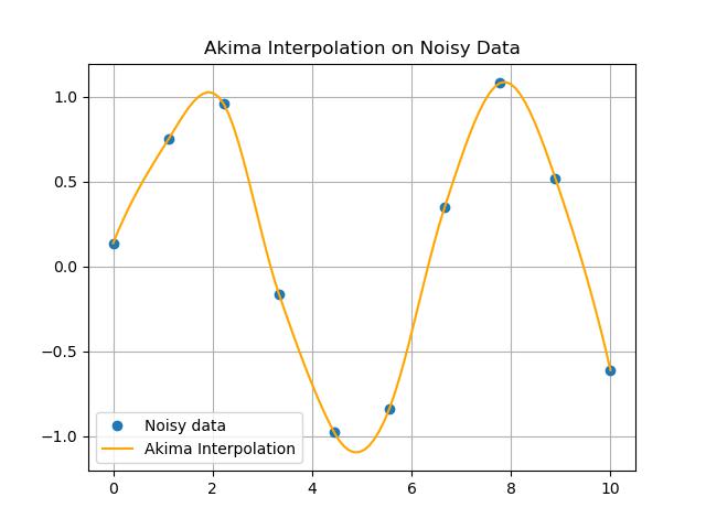
Interpolating Noisy Data

Interpolating noisy data can be challenging because noise can distort the underlying trends. Using Akima1DInterpolator() function can help to create a smooth approximation of the data while maintaining the overall shape. Heres an example of how to interpolate a noisy dataset using Akima interpolation. −

import numpy as np
from scipy.interpolate import Akima1DInterpolator
import matplotlib.pyplot as plt

# Original data points (with noise)
x = np.linspace(0, 10, 10)
y = np.sin(x) + np.random.normal(0, 0.1, x.shape)  # Add noise

# Create the Akima interpolator
akima = Akima1DInterpolator(x, y)

# Define new x values for interpolation
x_new = np.linspace(0, 10, 100)
y_new = akima(x_new)

# Plot the noisy data and the interpolation
plt.plot(x, y, 'o', label='Noisy data')
plt.plot(x_new, y_new, label='Akima Interpolation', color='orange')
plt.title('Akima Interpolation on Noisy Data')
plt.legend()
plt.grid()
plt.show()

Here is the output of the scipy.interpolate.Akima1DInterpolator() function working with Noisy data−