SciPy - interpolate.CubicHermiteSpline() Function

scipy.interpolate.CubicHermiteSpline() is a function used to construct a piecewise cubic Hermite interpolating spline which uses both function values and derivatives at given data points to produce a smooth curve. This method ensures that the curve passes through the specified points (x, y) and has specified slopes (dy/dx) at those points by maintaining continuity in both the function and its first derivative.

It is useful for interpolating data where the derivative is known or when smoothness of the first derivative is important. The resulting spline is continuous in both value and slope ensuring smooth transitions between segments.

Syntax

Following is the syntax of the function scipy.interpolate.CubicHermiteSpline() to perform cubic Hermite interpolation −

scipy.interpolate.CubicHermiteSpline(x, y, dydx, axis=0, extrapolate=None)

Parameters

Here are the parameters of the scipy.interpolate.CubicHermiteSpline() function −

• x: Array of independent variable values (data points). Must be strictly increasing.
• y:Array of dependent variable values (function values) at each point in x.
• dydx: Array of derivatives of y with respect to x at each point. Must have the same shape as y.
• axis (optional): The axis along which the interpolation is performed. Default value is 0.
• extrapolate(optional): If this parameter is set to True then it allows extrapolation beyond the provided x values. If False then it raises an error for out-of-bounds values. If default value i.e. None then extrapolates based on the first and last intervals.

Return Value

The scipy.interpolate.CubicHermiteSpline() function returns an instance of the CubicHermiteSpline class which represents a piecewise cubic Hermite interpolating spline.

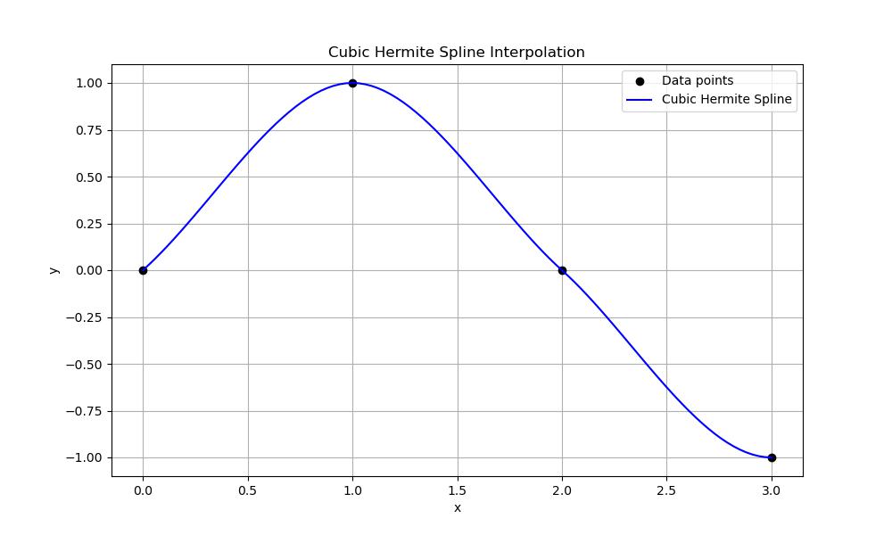
Basic Cubic Hermite Spline

Following is an example which uses the scipy.interpolate.CubicHermiteSpline() function to perform cubic Hermite interpolation. In this example we'll create a cubic Hermite spline using given data points and their slopes then evaluate the spline at specific points −

import numpy as np
import matplotlib.pyplot as plt
from scipy.interpolate import CubicHermiteSpline

# Define known data points
x = np.array([0, 1, 2, 3])
y = np.array([0, 1, 0, -1])  # Function values at x
dydx = np.array([1, 0, -1, 0])  # Slopes (derivatives) at x

# Create the cubic Hermite spline
spline = CubicHermiteSpline(x, y, dydx)

# Points where we want to evaluate the spline
xi = np.linspace(0, 3, 100)  # 100 points from 0 to 3
yi = spline(xi)  # Evaluate the spline

# Plot
plt.figure(figsize=(10, 6))
plt.plot(x, y, 'o', label='Data points', color='k')
plt.plot(xi, yi, label='Cubic Hermite Spline', color='b')
plt.title('Cubic Hermite Spline Interpolation')
plt.xlabel('x')

plt.ylabel('y')
plt.legend()
plt.grid(True)
plt.show()

Here is the output of the scipy.interpolate.CubicHermiteSpline() function −

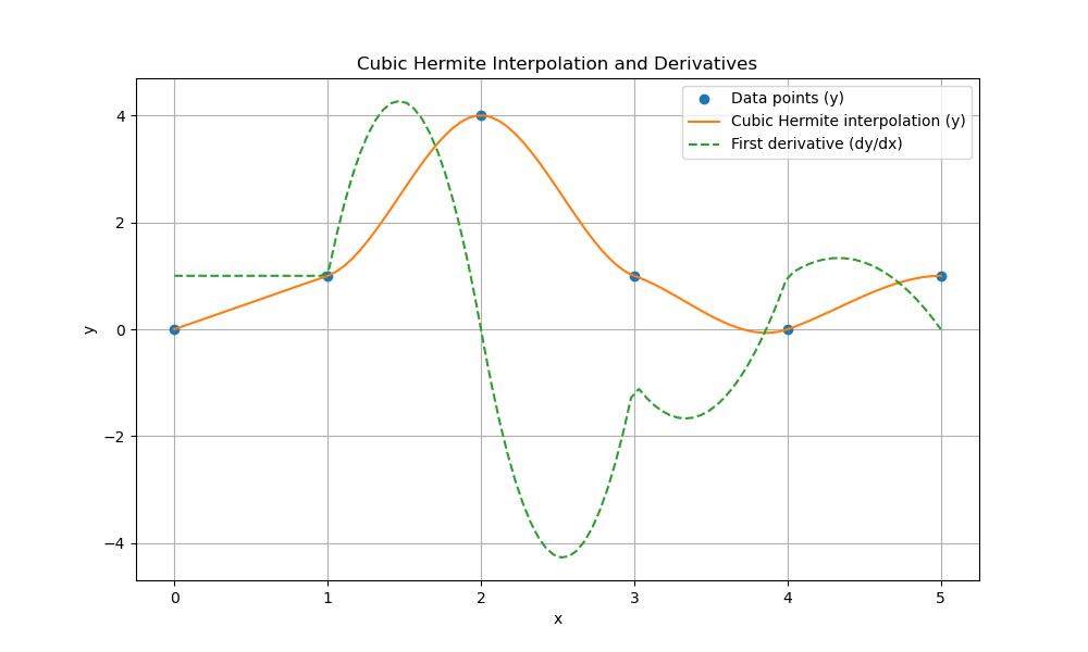
Evaluating Derivatives

Evaluating derivatives using cubic Hermite interpolation can be done using the CubicHermiteSpline() function from the scipy.interpolate module. This class not only allows us to interpolate values between given data points but also lets us to evaluate the first derivative of the interpolated function at any point within the interpolation range −

import numpy as np
import matplotlib.pyplot as plt
from scipy.interpolate import CubicHermiteSpline

# Define known data points (x) and their corresponding function values (y)
x = np.array([0, 1, 2, 3, 4, 5])
y = np.array([0, 1, 4, 1, 0, 1])

# Define the derivatives (dy/dx) at each point
dydx = np.array([1, 1, 0, -1, 1, 0])  # Sample derivatives

# Create the Cubic Hermite Spline interpolator
hermite_spline = CubicHermiteSpline(x, y, dydx)
# Define interpolation points
xi = np.linspace(0, 5, 100)

# Get the interpolated values
yi = hermite_spline(xi)

# Get the first derivative values at the interpolation points
dydxi = hermite_spline(xi, 1)  # The second argument is the derivative order

# Plot the results
plt.figure(figsize=(10, 6))
plt.plot(x, y, 'o', label='Data points (y)')
plt.plot(xi, yi, '-', label='Cubic Hermite interpolation (y)')
plt.plot(xi, dydxi, '--', label='First derivative (dy/dx)')
plt.legend()
plt.title('Cubic Hermite Interpolation and Derivatives')
plt.xlabel('x')
plt.ylabel('y')
plt.grid()
plt.show()

Following is the output of the scipy.interpolate.CubicHermiteSpline() function for finding the derivatives −

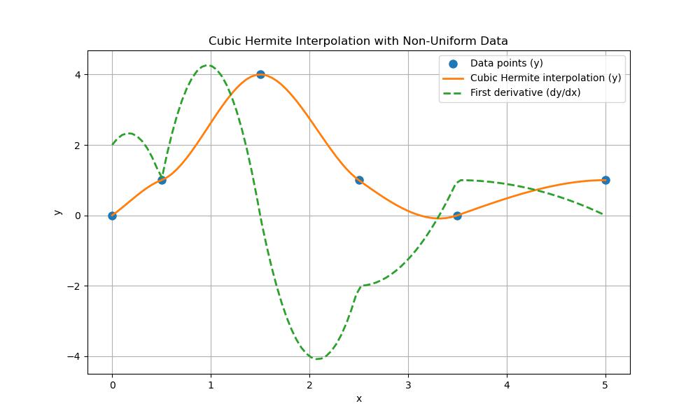
Non-Uniform Data and Slopes

In this example we'll define non-uniformly spaced data points along with their corresponding function values and slopes. We'll then use cubic Hermite interpolation to create an interpolated function and evaluate its derivatives −

import numpy as np
import matplotlib.pyplot as plt
from scipy.interpolate import CubicHermiteSpline

# Define non-uniformly spaced data points (x)
x = np.array([0, 0.5, 1.5, 2.5, 3.5, 5])  # Non-uniform spacing
y = np.array([0, 1, 4, 1, 0, 1])           # Corresponding function values

# Define the derivatives (dy/dx) at each point
dydx = np.array([2, 1, 0, -2, 1, 0])  # Sample slopes at the points

# Create the Cubic Hermite Spline interpolator
hermite_spline = CubicHermiteSpline(x, y, dydx)
# Define interpolation points (more dense for a smooth curve)
xi = np.linspace(0, 5, 100)

# Get the interpolated values
yi = hermite_spline(xi)

# Get the first derivative values at the interpolation points
dydxi = hermite_spline(xi, 1)  # The second argument is the derivative order

# Plot the results
plt.figure(figsize=(10, 6))
plt.plot(x, y, 'o', label='Data points (y)', markersize=8)
plt.plot(xi, yi, '-', label='Cubic Hermite interpolation (y)', linewidth=2)
plt.plot(xi, dydxi, '--', label='First derivative (dy/dx)', linewidth=2)
plt.title('Cubic Hermite Interpolation with Non-Uniform Data')
plt.xlabel('x')
plt.ylabel('y')
plt.legend()
plt.grid()
plt.show()

Following is the output of the scipy.interpolate.CubicHermiteSpline() function working with Non-Uniform Data −