SciPy - interpolate.BarycentricInterpolator() Function

scipy.interpolate.BarycentricInterpolator() is a Python function that performs polynomial interpolation using the Barycentric Lagrange interpolation formula. This method is particularly efficient and numerically stable for higher-degree polynomials compared to other forms of polynomial interpolation.

It constructs a polynomial that passes through a given set of points (xi, yi) by allowing for fast evaluation of the interpolating polynomial at new points. The BarycentricInterpolator() function avoids the direct computation of Lagrange polynomials by making it more stable when dealing with large data sets or high-degree polynomials. It is useful for smoothly estimating intermediate values between data points.

Syntax

Following is the syntax of the function scipy.interpolate.BarycentricInterpolator() to perform polynomial interpolation −

scipy.interpolate.BarycentricInterpolator(xi, yi=None, axis=0, *, wi=None, random_state=None)

Parameters

Here are the parameters of the scipy.interpolate.BarycentricInterpolator() function −

• xi(array-like): The x-coordinates of the data points. These points must be distinct.
• yi(array-like, optional): The corresponding y-coordinates of the function at each point in xi. If not provided then yi can be supplied later when the interpolator is called.
• axis(int, optional): The axis along which to interpolate when dealing with multi-dimensional yi arrays. The default value is 0.
• wi(array-like, optional): Barycentric weights for the data points. If not provided then the weights are calculated internally based on xi.
• random_state({None, int, numpy.random.Generator}, optional): Controls the reproducibility when generating random weights, if applicable. If random_state is an integer then it sets the seed, if its a Generator then its used for creating random numbers, if None then the global random generator is used.

Return Value

The scipy.interpolate.BarycentricInterpolator() function returns a callable object that can be used to perform interpolation at new data points.

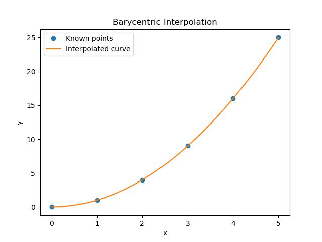
Basic Example

Following is the example which shows how to create a Barycentric interpolator for a set of points and use it to estimate values at new points with the help of the scipy.interpolate.BarycentricInterpolator() function −

import numpy as np
from scipy.interpolate import BarycentricInterpolator
import matplotlib.pyplot as plt

# Define known data points
x = np.array([0, 1, 2, 3, 4, 5])
y = np.array([0, 1, 4, 9, 16, 25])

# Create the interpolator
interp = BarycentricInterpolator(x, y)

# Define new points where interpolation is needed
x_new = np.linspace(0, 5, 100)
y_new = interp(x_new)

# Plot the results
plt.plot(x, y, 'o', label='Known points')
plt.plot(x_new, y_new, '-', label='Interpolated curve')
plt.legend()
plt.xlabel('x')
plt.ylabel('y')
plt.title('Barycentric Interpolation')
plt.show()

Here is the output of the scipy.interpolate.BarycentricInterpolator() function −

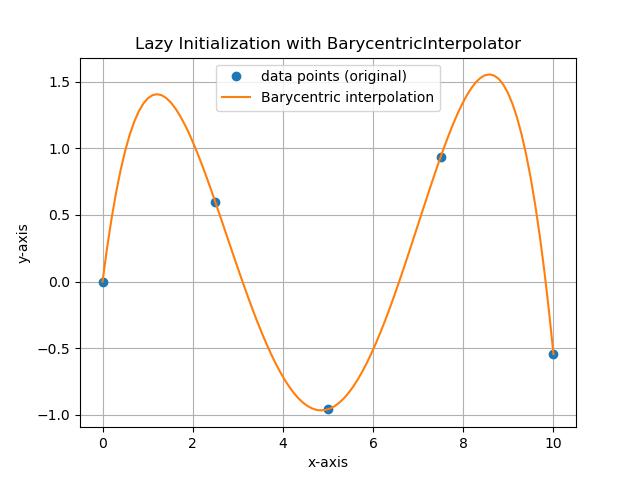
Lazy Initialization(Setting yi Later)

Lazy Initialization in the view of interpolation typically means that we can define the interpolation object first and then set the y values (yi) later which can be useful when we need to postpone specifying certain data until later in your workflow. Here is the example of it −

import numpy as np
import matplotlib.pyplot as plt
from scipy.interpolate import BarycentricInterpolator

# Step 1: Initialize known x-values (independent variable)
x = np.linspace(0, 10, num=5)  # x-coordinates

# Step 2: Lazy Initialization: Create a BarycentricInterpolator object without specifying yi (y-values)
interpolator = BarycentricInterpolator(x, np.zeros_like(x))  # Temporary yi of zeros

# Some other computations or data fetching
# Simulate a delay or other operations here
# Let's say we want to calculate yi using a function later

# Step 3: Now set the y-values later (Lazy Initialization of yi)
y = np.sin(x)  # Let's define yi as the sine of the x-values
interpolator = BarycentricInterpolator(x, y)  # Now initialize the function with yi

# Step 4: Define new x-values for interpolation
x_new = np.linspace(0, 10, num=100)

# Step 5: Interpolate for the new x-values
y_new = interpolator(x_new)

# Step 6: Plotting the results
plt.plot(x, y, 'o', label='data points (original)')
plt.plot(x_new, y_new, '-', label='Barycentric interpolation')
plt.title('Lazy Initialization with BarycentricInterpolator')
plt.xlabel('x-axis')
plt.ylabel('y-axis')
plt.legend()
plt.grid()
plt.show()

Here is the output of the scipy.interpolate.BarycentricInterpolator() function which is used for lazy initialization −

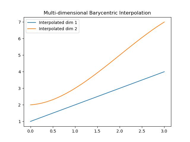
Multi-dimensional Interpolation

Here in this example if yi is multi-dimensional then we will specify the axis parameter to control how interpolation is applied −

import numpy as np
import matplotlib.pyplot as plt
from scipy.interpolate import BarycentricInterpolator

# Known data points
x = np.array([0, 1, 2, 3])
y = np.array([[1, 2], [2, 3], [3, 5], [4, 7]])

# Create the interpolator, specifying axis=0 (interpolating along the rows)
interp = BarycentricInterpolator(x, y, axis=0)

# New points for interpolation
x_new = np.linspace(0, 3, 50)
y_new = interp(x_new)

plt.plot(x_new, y_new[:, 0], label='Interpolated dim 1')
plt.plot(x_new, y_new[:, 1], label='Interpolated dim 2')
plt.legend()
plt.title('Multi-dimensional Barycentric Interpolation')
plt.show()

Following is the output of the scipy.interpolate.BarycentricInterpolator() function applied for multi-dimensional interpolation −